14  Adjusted Values

All adjustment series were pulled from FRED, the Federal Reserve Bank of St. Louis economic data platform https://fred.stlouisfed.org/. For series that have monthly observations, the first month of each year is the one used as the “year” value.

The data we use is listed below with the code necessary to pull it from FRED listed in parenthesis:

Show code
library(tidyverse)
library(cmapplot) # for recession line function
library(fredr)    # pulls data from FRED

# Values are in millions of dollars.
totals <- readxl::read_xlsx(
  "data/FY2025 Files/summary_file_FY2025_2026-01-23.xlsx",
  sheet = "aggregated_totals_long"
)
Show code
# Index data from FRED.
# You need an API key from the FRED website to pull the data.
# Store the key in your .Renviron file as FRED_API_KEY="your_key_here".

fred_api_key <- Sys.getenv("FRED_API_KEY")

if (fred_api_key == "") {
  stop("FRED_API_KEY is not set. Add it to your .Renviron file.")
}

fredr_set_key(fred_api_key)

series_ids <- c("ILNGSP", "CPIAUCSL", "WPSFD49406", "ILPOP", "A829RD3Q086SBEA")

fred_data <- map_dfr(
  series_ids,
  ~ fredr(
    series_id = .x,
    observation_start = as.Date("1900-01-01")
  )
) |>
  mutate(
    year = year(date),
    month = month(date)
  ) |>
  filter(year >= 1998) |>
  filter(
    (series_id == "CPIAUCSL" & month == 1) |
      (series_id == "WPSFD49406" & month == 1) |
      (series_id == "A829RD3Q086SBEA" & month == 1) |
      series_id == "ILPOP" |
      series_id == "ILNGSP"
  ) |>
  select(year, series_id, value) |>
  pivot_wider(
    id_cols = year,
    names_from = series_id,
    values_from = value
  )

write_csv(fred_data, "inputs/fred_data_for_index.csv")
Show code
adjustments <- read_csv("inputs/fred_data_for_index.csv")

totals2 <- totals |>
  left_join(adjustments, by = c("Year" = "year")) |>
  mutate(type = ifelse(type == "rev", "Revenue", "Expenditures"))

base_year <- 2025
current_year <- 2025

alea_theme <- function() {
  ggplot2::theme(
    legend.position = "right",
    legend.title = element_blank(),
    panel.background = ggplot2::element_blank(),
    panel.grid.minor.x = ggplot2::element_blank(),
    panel.grid.major.y = element_line(color = "grey"),
    panel.grid.minor.y = element_line(color = "grey", linetype = "dashed"),
    axis.ticks = element_line(color = "gray"),
    axis.ticks.x = element_blank()
  )
}

theme_set(alea_theme())

# This keeps an all-missing year from becoming zero after summarize().
sum_keep_na <- function(x) {
  if (all(is.na(x))) {
    NA_real_
  } else {
    sum(x, na.rm = TRUE)
  }
}

get_base_value <- function(data, index_col, base_year = 2025) {
  data |>
    filter(Year == base_year) |>
    distinct(.data[[index_col]]) |>
    pull(.data[[index_col]]) |>
    first()
}

make_base_plot <- function(plot_data, title, y_label, y_scale) {
  ggplot(plot_data, aes(x = Year, y = adj_value, group = type, color = type, lty = type)) +
    geom_recessions(text = FALSE, update = recessions) +
    geom_line(lwd = 1) +
    y_scale +
    scale_color_manual(values = c("Revenue" = "black", "Expenditures" = "red")) +
    scale_x_continuous(
      expand = c(0, 0),
      limits = range(plot_data$Year, na.rm = TRUE),
      breaks = sort(unique(c(1998, 2005, 2010, 2015, 2020, max(plot_data$Year, na.rm = TRUE))))
    ) +
    labs(
      title = title,
      y = y_label,
      x = NULL
    ) +
    theme_minimal() +
    theme(legend.title = element_blank())
}

update_recessions <- function(url = NULL, quietly = FALSE) {
  if (is_null(url) | missing(url)) {
    url <- "https://data.nber.org/data/cycles/business_cycle_dates.json"
  }

  start_char <- end_char <- start_date <- end_date <- ongoing <- index <- peak <- trough <- NULL

  tryCatch({
    recessions <- jsonlite::fromJSON(url) |>
      dplyr::slice(-1) |>
      dplyr::mutate(
        start_date = as.Date(peak),
        end_date = as.Date(trough),
        start_char = format(start_date, "%b %Y"),
        end_char = format(end_date, "%b %Y")
      ) |>
      dplyr::arrange(start_date) |>
      mutate(index = row_number()) |>
      mutate(
        ongoing = case_when(
          is.na(end_date) & index == max(.$index) ~ TRUE,
          TRUE ~ FALSE
        ),
        end_date = case_when(
          ongoing ~ as.Date("2200-01-01"),
          TRUE ~ end_date
        ),
        end_char = case_when(
          ongoing ~ "Ongoing",
          TRUE ~ end_char
        )
      ) |>
      select(start_char, end_char, start_date, end_date, ongoing)

    if (!quietly) {
      message("Successfully fetched from NBER")
    }

    recessions
  },
  error = function(cond) {
    if (!quietly) {
      message("WARNING: Fetch or processing failed. `NULL` returned.")
    }
    NULL
  })
}

recessions <- update_recessions()

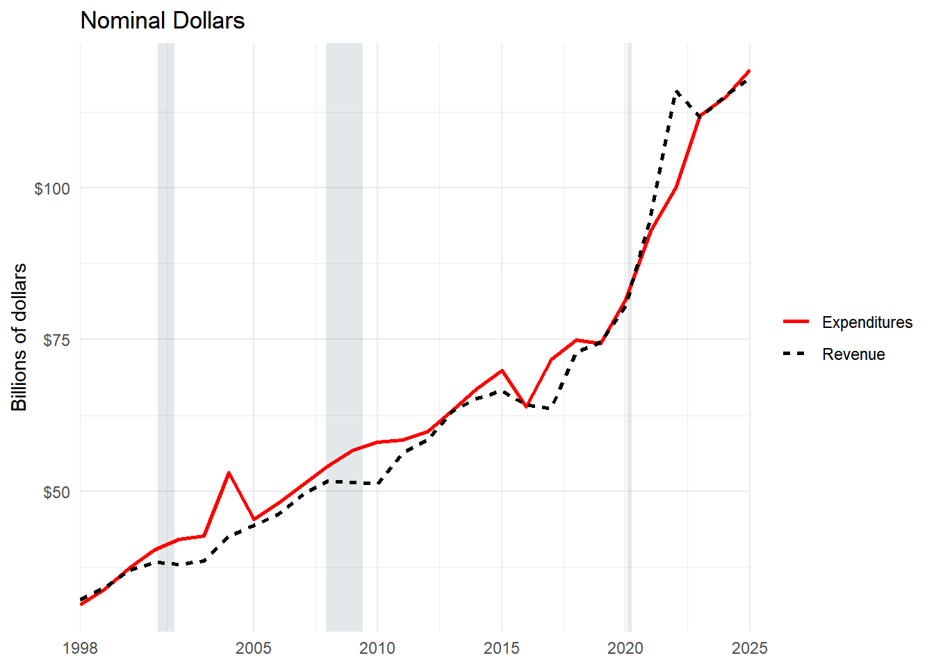
15 Nominal Dollars

Show code
plot_data <- totals2 |>
  mutate(adj_value = Dollars / 1000) |>
  group_by(Year, type) |>
  summarize(adj_value = sum_keep_na(adj_value), .groups = "drop") |>
  filter(!is.na(adj_value))

make_base_plot(
  plot_data = plot_data,
  title = "Nominal Dollars",
  y_label = "Billions of dollars",
  y_scale = scale_y_continuous(labels = scales::label_dollar())
)

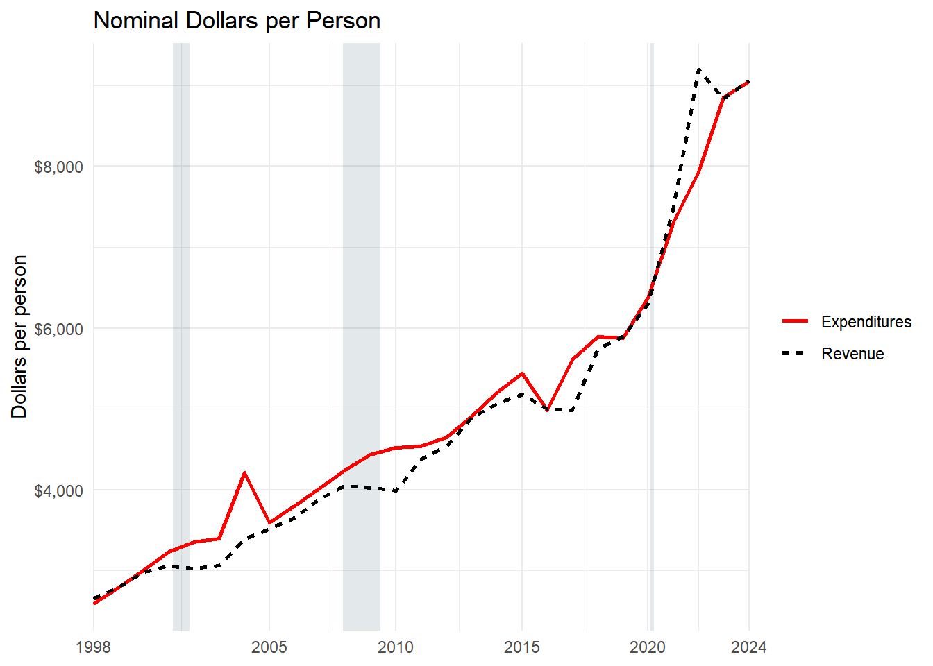
16 Nominal Dollars per Person

Show code
plot_data <- totals2 |>
  mutate(adj_value = Dollars / ILPOP * 1000) |>
  group_by(Year, type) |>
  summarize(adj_value = sum_keep_na(adj_value), .groups = "drop") |>
  filter(!is.na(adj_value))

make_base_plot(
  plot_data = plot_data,
  title = "Nominal Dollars per Person",
  y_label = "Dollars per person",
  y_scale = scale_y_continuous(labels = scales::label_dollar())
)

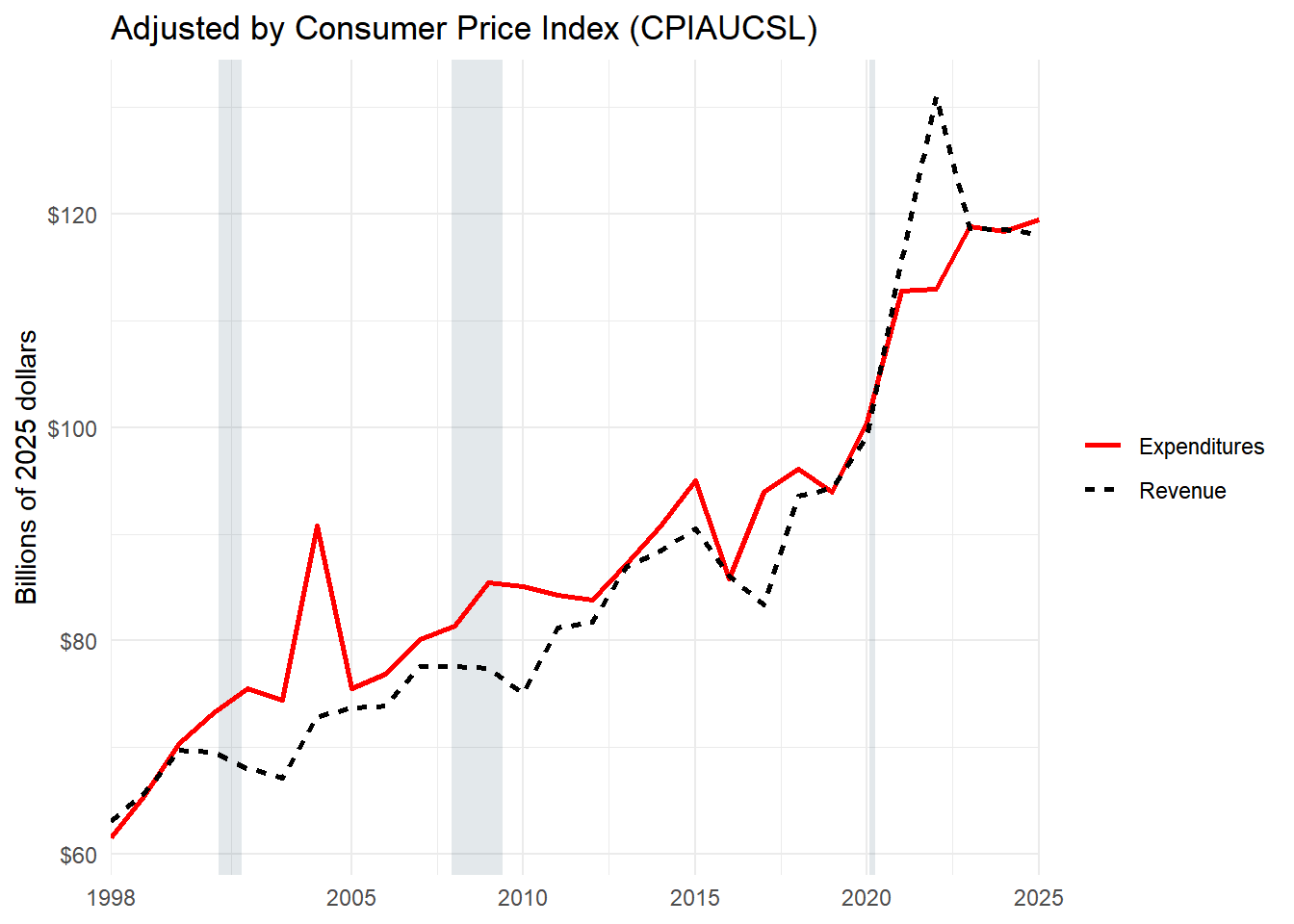
17 Adjusted by Consumer Price Index

Show code
cpi_base <- get_base_value(totals2, "CPIAUCSL", base_year)

plot_data <- totals2 |>
  mutate(adj_value = Dollars * (cpi_base / CPIAUCSL) / 1000) |>
  group_by(Year, type) |>
  summarize(adj_value = sum_keep_na(adj_value), .groups = "drop") |>
  filter(!is.na(adj_value))

make_base_plot(
  plot_data = plot_data,
  title = "Adjusted by Consumer Price Index (CPIAUCSL)",
  y_label = paste0("Billions of ", base_year, " dollars"),
  y_scale = scale_y_continuous(labels = scales::label_dollar())
)

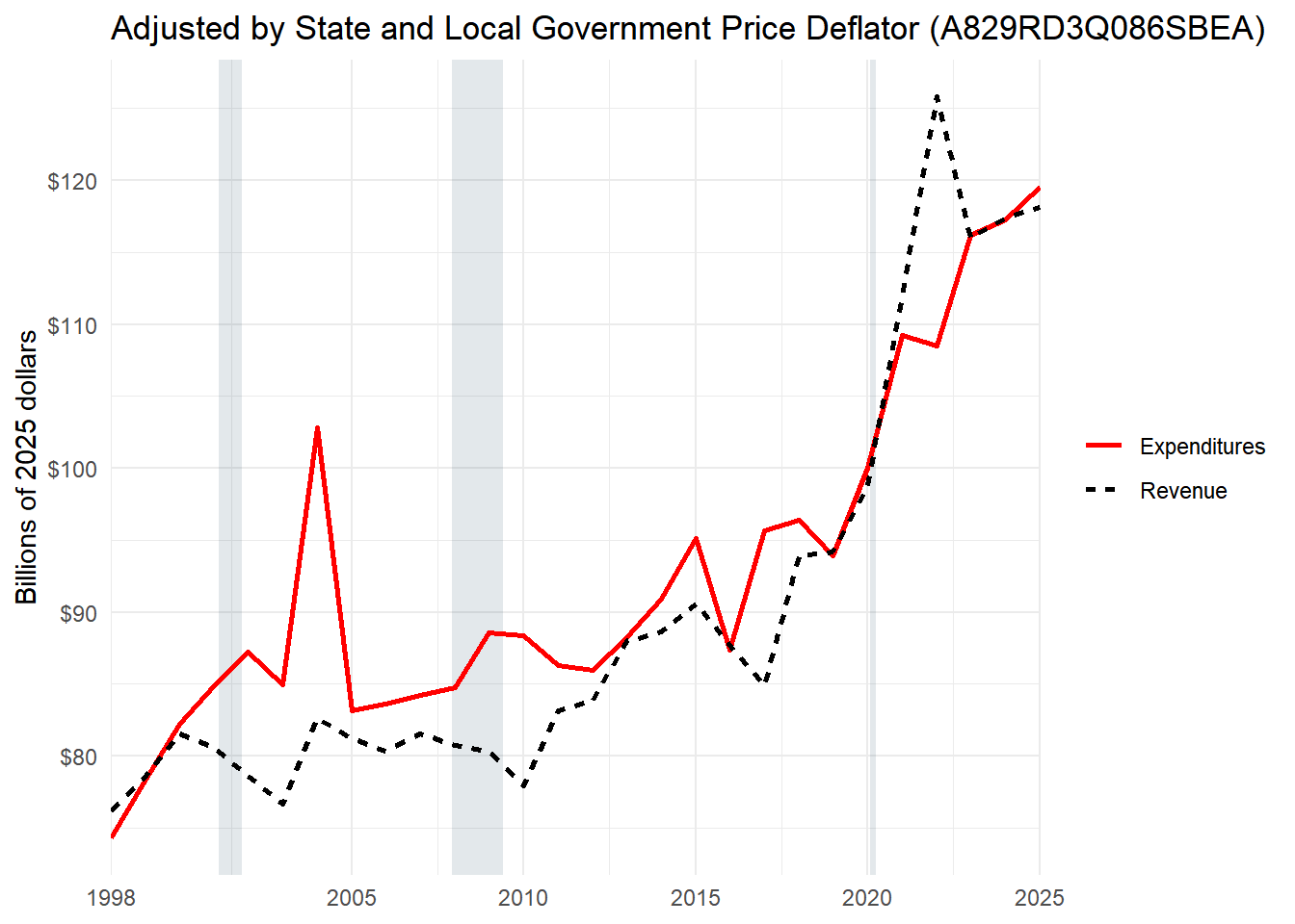
18 Adjusted by State and Local Government Price Deflator

This plot follows the Excel formula nominal value * S&L price deflator base-year value / S&L price deflator current-year value. The output is plotted in billions of base-year dollars.

Show code
sbea_base <- get_base_value(totals2, "A829RD3Q086SBEA", base_year)

plot_data <- totals2 |>
  mutate(adj_value = Dollars * (sbea_base / A829RD3Q086SBEA) / 1000) |>
  group_by(Year, type) |>
  summarize(adj_value = sum_keep_na(adj_value), .groups = "drop") |>
  filter(!is.na(adj_value))

make_base_plot(
  plot_data = plot_data,
  title = "Adjusted by State and Local Government Price Deflator (A829RD3Q086SBEA)",
  y_label = paste0("Billions of ", base_year, " dollars"),
  y_scale = scale_y_continuous(labels = scales::label_dollar())
)

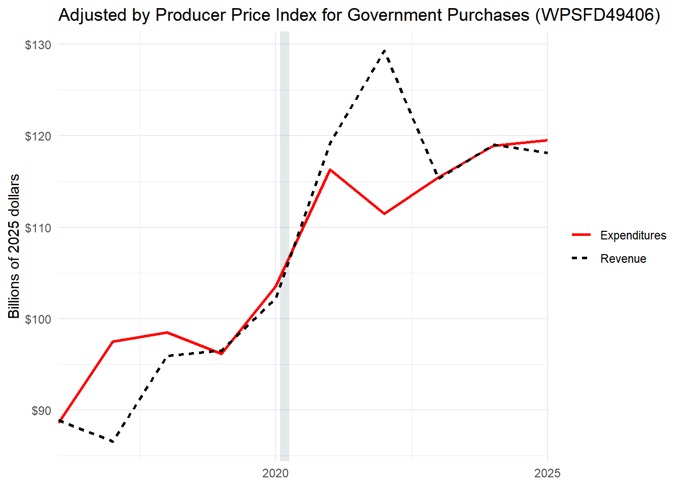
19 Adjusted by Producer Price Index for Government Purchases

The PPI series starts later than the other series, so years with missing PPI values are dropped from this plot.

Show code
ppi_base <- get_base_value(totals2, "WPSFD49406", base_year)

plot_data <- totals2 |>
  mutate(adj_value = Dollars * (ppi_base / WPSFD49406) / 1000) |>
  group_by(Year, type) |>
  summarize(adj_value = sum_keep_na(adj_value), .groups = "drop") |>
  filter(!is.na(adj_value))

make_base_plot(
  plot_data = plot_data,
  title = "Adjusted by Producer Price Index for Government Purchases (WPSFD49406)",
  y_label = paste0("Billions of ", base_year, " dollars"),
  y_scale = scale_y_continuous(labels = scales::label_dollar())
)

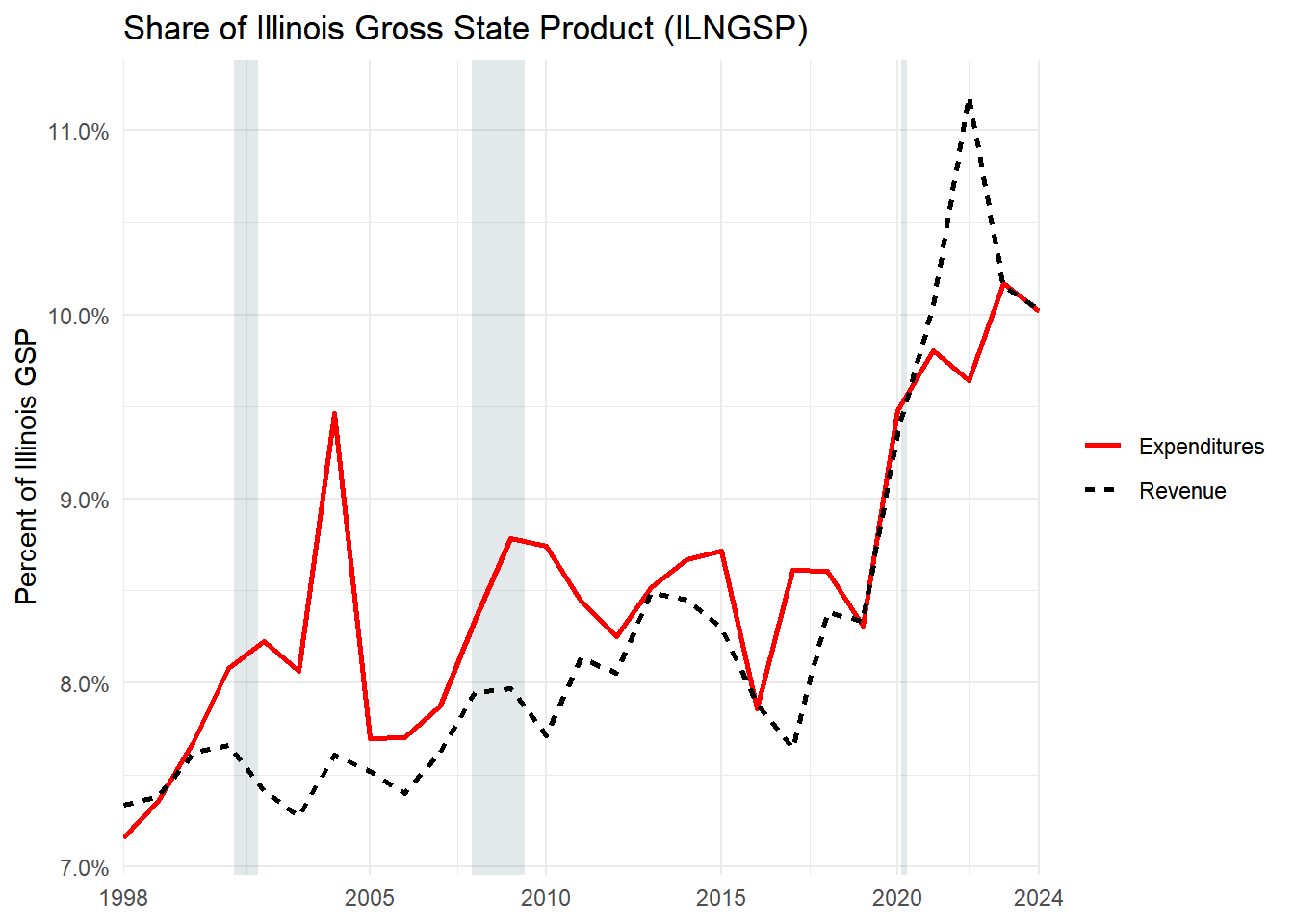
20 Share of Illinois Gross State Product

Show code
plot_data <- totals2 |>
  mutate(adj_value = Dollars / ILNGSP) |>
  group_by(Year, type) |>
  summarize(adj_value = sum_keep_na(adj_value), .groups = "drop") |>
  filter(!is.na(adj_value))

make_base_plot(
  plot_data = plot_data,
  title = "Share of Illinois Gross State Product (ILNGSP)",
  y_label = "Percent of Illinois GSP",
  y_scale = scale_y_continuous(labels = scales::label_percent(accuracy = 0.1))
)