3 Pension Costs Included within Department Expenditures

In previous reports, a expenditure category was created to represent all Pension spending. It was created by removing pension expenditures out of the agencies that that had the expenses in order to highlight the amount that was spent on pensions.

As of the FY2024 report, pension expenditures will remain in the agency that has the pension expenses to better represent the total cost of providing a service to the public.

However, we thought that readers also might be interested in total pension spending during current and past years. We have added a separate table showing this information but emphasize that pension spending is already incorporated in other spending categories and should not be added to the total shown in Table 1 of the report.

Code

knitr::opts_chunk$set(echo = TRUE, warning = FALSE, message = FALSE)

library(tidyverse)
library(formatR)
library(lubridate)
library(scales)
library(kableExtra)
library(ggplot2)
library(readxl)
library(janitor)
#devtools::install_github("CMAP-REPOS/cmapplot")
library(cmapplot)


move_to_last <- function(df, n) df[c(setdiff(seq_len(nrow(df)), n), n), ]


current_year <- 2025 # fiscal year, not calendar year
past_year=current_year-1

rev_temp <- read_csv(paste0("data/FY", current_year, " Files/rev_temp.csv"))

exp_temp <- read_csv(paste0("data/FY", current_year, " Files/exp_temp.csv"))

3.1 Modify Expenditure File

3.1.1 Tax refunds

For more details on refund items, see Chapter 12.

Aggregate expenditures:

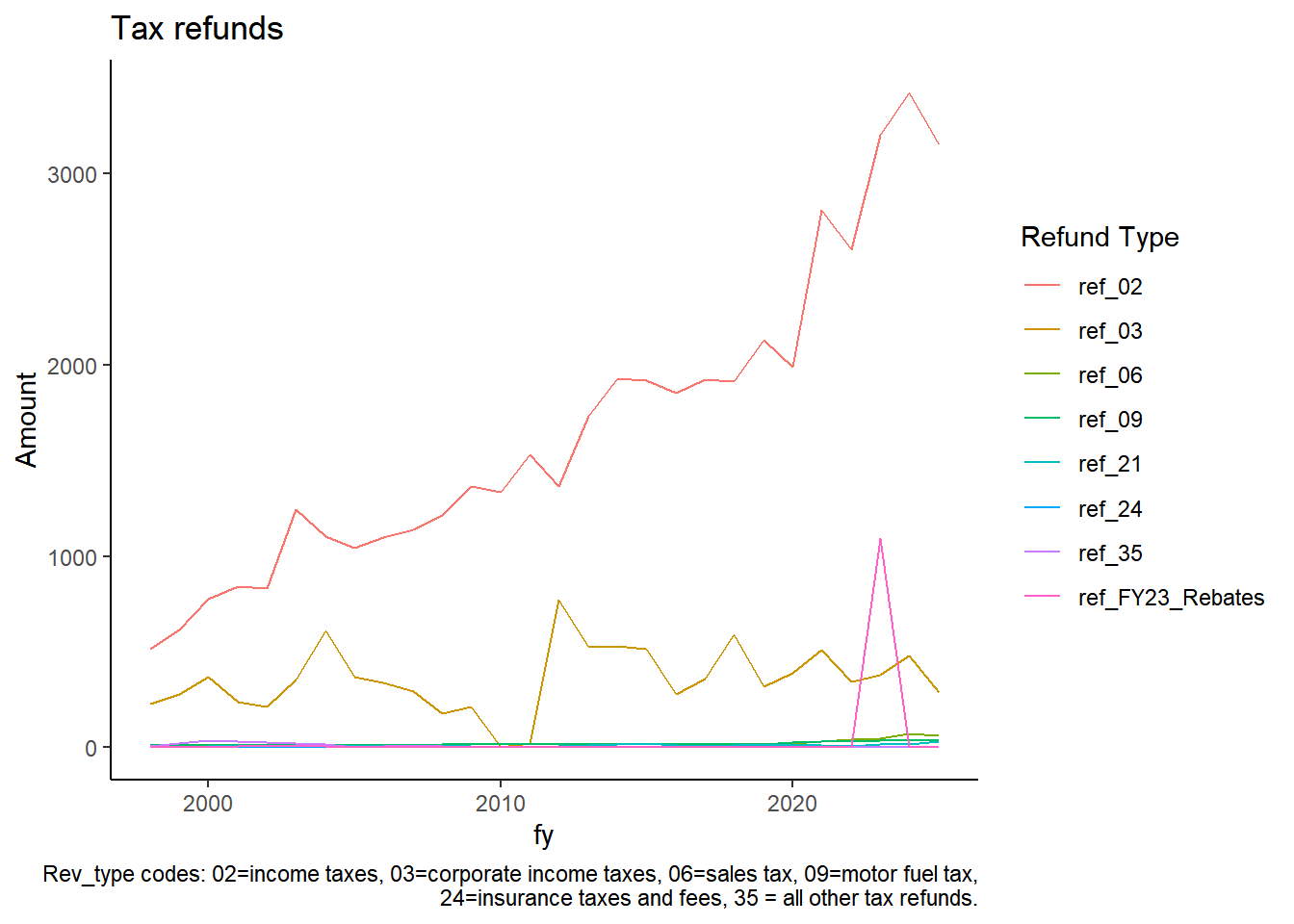
Code refunds to match the rev_type codes (02=income taxes, 03=corporate income taxes, 06=sales tax, 09=motor fuel tax, 24=insurance taxes and fees, 35 = all other tax refunds).

Ideally the money going in and out of the funds used for refunds would be approximately equal. If equal, would drop from Fiscal Futures analysis so that Revenue reflects the amount of money the state gets to keep (and the local portion that becomes the local govt transfer)

Code

# What we want: To exclude refunds as expenditures from our expenditure totals.
# Exclude funds that hold refund funds from both revenue and expenditure sides
# Revenue neutral unless budget tricks are occurring
# still want to examine refunds over time to compare to past years calculations


tax_refund_long <- exp_temp %>%  
  
  # filter out only refund objects
    # keeps these objects which represent revenue, insurance, treasurer,and financial and professional reg tax refunds
  filter(fund != "0401" & # fund != "0401" # removes State Trust Funds
           (object == "9900" | object=="9910"|object=="9921"|object=="9923"|object=="9925")) %>%
  
  # add revenue category numbers
  mutate(refund = case_when(
    object == "9900" ~ "FY23_Rebates",      # part of COVID relief
    fund=="0278" & sequence == "00" ~ "02", # for income tax refund
    fund=="0278" & sequence == "01" ~ "03", # tax administration and enforcement and tax operations become corporate income tax refund
    fund == "0278" & sequence == "02" ~ "02",
    object=="9921" ~ "21",                # inheritance tax and estate tax refund appropriation
    object=="9923" ~ "09",                # motor fuel tax refunds
    obj_seq_type == "99250055" ~ "06",    # sales tax refund
    fund=="0378" & object=="9925" ~ "24", # insurance privilege tax refund
    (fund=="0001" & object=="9925") | 
      (object=="9925" & fund == "0384" & 
         fy == 2023) ~ "35",               # all other taxes
    T ~ "CHECK"))                       # if none of the items above apply to the observations, then code them as CHECK 

    
exp_temp <- left_join(exp_temp, tax_refund_long) %>%
  mutate(refund = ifelse(is.na(refund),"not refund", as.character(refund)))

Code

tax_refund <- tax_refund_long %>% 
  group_by(refund, fy)%>%
  summarize(refund_amount = sum(expenditure, na.rm = TRUE)/1000000) %>%
  pivot_wider(names_from = refund, values_from = refund_amount, names_prefix = "ref_") %>%
  mutate_all(~replace_na(.,0)) %>%
  arrange(fy)

tax_refund %>%
  pivot_longer(c(ref_02:ref_35, ref_FY23_Rebates), names_to = "Refund Type", values_to = "Amount") %>%
  ggplot()+
  theme_classic()+
  geom_line(aes(x=fy,y=Amount, group = `Refund Type`, color = `Refund Type`))+
  labs(title = "Refund Types",
       caption = "Refunds are excluded from Expenditure totals and instead subtracted from Revenue totals") +
  labs(title = "Tax refunds",
       caption = "Rev_type codes: 02=income taxes, 03=corporate income taxes, 06=sales tax, 09=motor fuel tax,
       24=insurance taxes and fees, 35 = all other tax refunds." )

# remove the items we recoded in tax_refund_long
# exp_temp <- exp_temp %>% filter(refund == "not refund")

For FY23, the one-time abatement, object 9900, is included as an expenditure item within the Department of Revenue.

Code

# manually adds the abatements as expenditure item and keeps on expenditure side.
# otherwise ignored since it is in fund 0278 and 
exp_temp <- exp_temp %>%
  mutate(in_ff = ifelse(object == 9900, 1, in_ff))

3.1.2 Pension Expenditures

State pension contributions for TRS and SURS are largely captured with object=4431. (State payments into pension fund). State payments to the following pension systems:

Teachers Retirement System (TRS) Agency 493 –> K-12 Education (Group = 959)
New POB bond in 2019: Accelerated Bond Fund paid benefits in advance as lump sum
State Employee Retirement System (SERS) Agency 589 –> SERS Agency 589 - Note: Object 4431 does not have SERS expenditures in it. Those are only in object 116X objects
State University Retirement System (SURS) Agency 693 –> University Education (Group = 960)
Judges Retirement System (JRS) Agency 275 –> Judicial (Group = 920)
General Assembly Retirement System (GARS) –> Legislative (Group 910)

There are also “Other Post-Employment Benefits” (OPEBs). Expenditure object 4430 is for retirement benefits.

While it is good to know the overall cost of pensions for the state, if you want to know the true cost of providing services, pension and other benefit costs should be included in the department that is paying employees to provide those services.

Change in pension coding in chunk below:

Code

exp_temp <-  exp_temp %>% 
  arrange(fund) %>%
  mutate(pension = case_when( 
    
    ## Commented out line below:
     (object=="4431") ~ 1, # 4431 = easy to find pension payments INTO fund
    

    
    (object=="1298" &  # Purchase of Investments, Normally excluded
       (fy==2010 | fy==2011) & 
       (fund=="0477" | fund=="0479" | fund=="0481")) ~ 3, #judges retirement OUT of fund
    # state borrowed money from pension funds to pay for core services during 2010 and 2011. 
    # used to fill budget gap and push problems to the future. 
    
    fund == "0319" ~ 4, # pension stabilization fund
    TRUE ~ 0) )

Code

# special accounting of pension obligation bond (POB)-funded contributions to JRS, SERS, GARS, TRS 

exp_temp <- exp_temp %>% 
  # change object for 2010 and 2011, retirement expenditures were bond proceeds and would have been excluded
  mutate(object = ifelse((pension > 0 & in_ff == "0"), "4431", object)) %>% 
  # changes weird teacher & judge retirement system  pensions object to normal pension object 4431
  mutate(pension =  ifelse(pension > 0 & in_ff == "0", 6, pension)) %>% # coded as 6 if it was supposed to be excluded. 
  mutate(in_ff = ifelse(pension > 0, "1", in_ff))



# # all other pensions objects  codes get agency code 901 for State Pension Contributions
# exp_temp <- exp_temp %>% 
#   mutate(agency = ifelse(pension > 0, "901", as.character(agency)),
#          agency_name = ifelse(agency == "901", "State Pension Contributions", as.character(agency_name)))

Can also be thought of past commitments vs current contributions.

Where past commitments in the form of pension benefits paid out.

Current Employees vs Retired Employees

Current Employees: - Group Insurance Benefits

Retired Employees: - Deferred Compensation
- Medicare Retirees and Survivors of State of Illinois Employees Group Insurance Program (SEGIP)
- Part of Medicare

Code

exp_temp|>
  filter(fy==2024) |>
  filter((appr_org=="01" | appr_org == "65" | appr_org=="88") & (object=="4900" | object=="4400") )|> 
  group_by(agency, agency_name) |> # separates CHIP from health and human services and saves it as Medicaid
  summarize(expenditure = sum(expenditure))

Drop all cash transfers between funds, statutory transfers, and purchases of investments from expenditure data.

Code

transfers_drop <- exp_temp %>% filter(
  agency == "799" | # statutory transfers
           object == "1993" |  # interfund cash transfers
           object == "1298") # purchase of investments
transfers_drop # items being dropped,

Code

# always check to make sure you aren't accidentally dropping something of interest.

exp_temp <- anti_join(exp_temp, transfers_drop)

3.1.3 State employee healthcare costs

Commented out line of code that seperates healthcare costs. This should keep healthcare costs in the agency, similar to the change that was made for pensions.

Also not grouping the agencies below into “Other Departments” until final steps of aggregation. Smallest agencies will be combined into Other Departments for final summary tables.

agency=="507"|  agency=="442" | agency=="445" | agency=="452" |agency=="458" | agency=="497" ~ "948", # other departments

When healthcare costs are not manually separated into their own category, it looks like the costs shift to many of the smaller departments, such as:

GOMB (507)
Human Rights (442)
Illinois Power Agency (445)
Labor (452)
State Lottery (458)
Veteran’s Affairs (497)

Code

#if observation is a group insurance contribution, then the expenditure amount is set to $0 (essentially dropped from analysis)

# pretend eehc is named group_insurance_contribution or something like that
# eehc coded as zero implies that it is group insurance
# if eehc=0, then expenditures are coded as zero for group insurance to avoid double counting costs


exp_temp <- exp_temp %>% 
  mutate(eehc = ifelse(
    # group insurance contributions for 1998-2005 and 2013-present
   fund == "0001" & (object == "1180" | object =="1900") & agency == "416" & appr_org=="20", 0, 1) )%>% 
  
  mutate(eehc = ifelse(
    # group insurance contributions for 2006-2012
    fund == "0001" & object == "1180" & agency == "478" 
    & appr_org=="80", 0, eehc) )%>%
    
   # group insurance contributions from road fund
  # coded with 1900 for some reason??
    mutate(eehc = ifelse(
      fund == "0011" & object == "1900" & 
        agency == "416" & appr_org=="20", 0, eehc) ) %>%
  
  mutate(expenditure = ifelse(eehc=="0", 0, expenditure)) %>%

  mutate(agency = case_when(
    ## turns specific items into State Employee Healthcare (agency=904)
      fund=="0907" & (agency=="416" & appr_org=="20") ~ "904",   # central management Bureau of benefits using health insurance reserve
      fund=="0907" & (agency=="478" & appr_org=="80") ~ "904",   # agency = 478: healthcare & family services using health insurance reserve - stopped using this in 2012
       TRUE ~ as.character(agency))) %>%
  
  mutate(agency_name = ifelse(
    agency == "904", "STATE EMPLOYEE HEALTHCARE", as.character(agency_name)),
         in_ff = ifelse(agency == "904", 1, in_ff),
         group = ifelse(agency == "904", "904", as.character(agency)))  
# creates group variable

# Default group = agency number

healthcare_costs <- exp_temp %>% filter(group == "904")

Code

exp_temp <- exp_temp %>% mutate(
  agency = case_when(fund=="0515" & object=="4470" & type=="08" ~ "971", # income tax to local governments
                     fund=="0515" & object=="4491" & type=="08" & sequence=="00" ~ "971", # object is shared revenue payments
                     fund=="0802" & object=="4491" ~ "972", #pprt transfer
                     fund=="0515" & object=="4491" & type=="08" & sequence=="01" ~ "976", #gst to local
                     fund=="0627" & object=="4472"~ "976" , # public transportation fund but no observations exist
                     fund=="0648" & object=="4472" ~ "976", # downstate public transportation, but doesn't exist
                     fund=="0515" & object=="4470" & type=="00" ~ "976", # object 4470 is grants to local governments
                    object=="4491" & (fund=="0188"|fund=="0189") ~ "976",
                     fund=="0187" & object=="4470" ~ "976",
                     fund=="0186" & object=="4470" ~ "976",
                    object=="4491" & (fund=="0413"|fund=="0414"|fund=="0415")  ~ "975", #mft to local
                  fund == "0952"~ "975", # Added Sept 29 2022 AWM. Transportation Renewal MFT
                    TRUE ~ as.character(agency)),
  
  agency_name = case_when(agency == "971"~ "INCOME TAX 1/10 TO LOCAL",
                          agency == "972" ~ "PPRT TRANSFER TO LOCAL",
                          agency == "975" ~ "MFT TO LOCAL",
                          agency == "976" ~ "GST TO LOCAL",
                          TRUE~as.character(agency_name)),
  group = ifelse(agency>"970" & agency < "977", as.character(agency), as.character(group)))

Code

transfers_long <- exp_temp %>% 
  filter(group == "971" |group == "972" | group == "975" | group == "976")


transfers <- transfers_long %>%
  group_by(fy, group ) %>%
  summarize(sum_expenditure = sum(expenditure)/1000000) %>%
  pivot_wider(names_from = "group", values_from = "sum_expenditure", names_prefix = "exp_" )

exp_temp <- anti_join(exp_temp, transfers_long)


dropped_inff_0 <- exp_temp %>% filter(in_ff == 0)

exp_temp <- exp_temp %>% filter(in_ff == 1) # drops in_ff = 0 funds AFTER dealing with net-revenue above

Code

debt_drop <- exp_temp %>% 
  filter(object == "8841" |  object == "8811")  
# escrow  OR  principle

#debt_drop %>% group_by(fy) %>% summarize(sum = sum(expenditure)) %>% arrange(-fy)


debt_keep <- exp_temp %>% 
  filter(fund != "0455" & (object == "8813" | object == "8800" )) 
# examine the debt costs we want to include

#debt_keep %>% group_by(fy) %>% summarize(sum = sum(expenditure)) %>% arrange(-fy) 


exp_temp <- anti_join(exp_temp, debt_drop) 
exp_temp <- anti_join(exp_temp, debt_keep)

debt_keep <- debt_keep %>%
  mutate(
    agency = ifelse(fund != "0455" & (object == "8813" | object == "8800"), "903", as.character(agency)),
    group = ifelse(fund != "0455" & (object == "8813" | object == "8800"), "903", as.character(group)),
    in_ff = ifelse(group == "903", 1, as.character(in_ff)))

debt_keep_yearly <- debt_keep %>% 
  group_by(fy, group) %>% 
  summarize(debt_cost = sum(expenditure,na.rm=TRUE)/1000000) %>% 
  select(-group)

3.1.4 Add Other Fiscal Future group codes

Code

exp_temp <- exp_temp %>%
  #mutate(agency = as.numeric(agency) ) %>%
  # arrange(agency)%>%
  mutate(
    group = case_when(
      agency>"100"& agency<"200" ~ "910", # legislative
      
      agency == "528"  | (agency>"200" & agency<"300") ~ "920", # judicial
      
      ######################################################
      # Not used if we are not separating pension costs!!
      # pension > 0  ~ "901", # pensions
      
      ## New CODE: April 23rd, 2025:
      agency == "593" ~ "959", #  TRS becomes part of K-12 costs
      agency == "594" ~ "959",   # TRS
      agency == "589" ~ "948", # SERS becomes part of "Other Agencies"
      agency == "693" ~ "960", # SURS becomes part of group 960
      agency == "275" ~ "920",  # JRS becomes part of group 920
      agency == "131" ~  "910", # GARS becomes part of Group 910
      ######################################################
      
      (agency>"309" & agency<"400") ~ "930",    # elected officers: Governor, lt gov, attorney general, sec. of state, comptroller, treasurer
      
      agency == "586" ~ "959", # create new K-12 group

      agency=="402" | agency=="418" | agency=="478" | agency=="444" | agency=="482" ~ as.character(agency), # aging, CFS, HFS, human services, public health
      
      T ~ as.character(group))
    ) %>%      

  
  mutate(group = case_when(
    agency=="478" & (appr_org=="01" | appr_org == "65" | appr_org=="88") & (object=="4900" | object=="4400") ~ "945", # separates CHIP from health and human services and saves it as Medicaid
    
    agency == "586" & fund == "0355" ~ "945",  # 586 (Board of Edu) has special education which is part of medicaid
    
    # OLD CODE: agency == "586" & appr_org == "18" ~ "945", # Spec. Edu Medicaid Matching
    
    agency=="425" | agency=="466" | agency=="546" | agency=="569" | agency=="578" | agency=="583" | agency=="591" | agency=="592" | agency=="493" | agency=="588" ~ "941", # public safety & Corrections
    
    agency=="420" | agency=="494" |  agency=="406" | agency=="557" ~ as.character(agency), # econ devt & infra, tollway
    
    agency=="511" | agency=="554" | agency=="574" | agency=="598" ~ "946",  # Capital improvement
    
    agency=="422" | agency=="532" ~ as.character(agency), # environment & nat. resources
    
    agency=="440" | agency=="446" | agency=="524" | agency=="563"  ~ "944", # business regulation
    
    agency=="492" ~ "492", # revenue
    
    agency == "416" ~ "416", # central management services
    agency=="448" & fy > 2016 ~ "416", #add DoIT to central management 
    
    T ~ as.character(group))) %>%
  
  
  mutate(group = case_when(
    # agency=="684" | agency=="691"  ~ as.character(agency), # moved under higher education in next line. 11/28/2022 AWM
    
    agency=="692" | agency == "693" | agency=="695" | agency == "684" |agency == "691" | (agency>"599" & agency<"677") ~ "960", # higher education
    
    agency=="427"  ~ as.character(agency), # employment security
    
############################ 
# Leaving these agencies as their own agency number for now. 
# Had been coded to "Other departments" Group 948
# - GOMB (507)  
# - Human Rights (442)  
# - Illinois Power Agency (445)  
# - Labor (452)   
# - State Lottery (458)   
# - Veteran's Affairs (497) 

  #     agency=="507" | agency=="442" | agency=="445" | agency=="452" |agency=="458" | agency=="497" ~ as.character(agency), # Were included within "other departments"
    
    agency=="507"|  agency=="442" | agency=="445" | agency=="452" |agency=="458" | agency=="497" ~ "948", # other departments
###########################################
    

# other boards & Commissions
    agency=="503" | agency=="509" | agency=="510" | agency=="565" |agency=="517" | agency=="525" | agency=="526" | agency=="529" | agency=="537" | agency=="541" | agency=="542" | agency=="548" |  agency=="555" | agency=="558" | agency=="559" | agency=="562" | agency=="564" | agency=="568" | agency=="579" | agency=="580" | agency=="587" | agency=="590" | agency=="527" | agency=="585" | agency=="567" | agency=="571" | agency=="575" | agency=="540" | agency=="576" | agency=="564" | agency=="534" | agency=="520" | agency=="506" | agency == "533" ~ "949", 
    
  #   # Other Departments
  #   agency=="131" |
  # #  agency=="275" | #JRS
  # #  agency=="589" | #SERS
  #  # agency=="593"|  # TRS
  # #  agency=="594"| # Also TRS
  # #  agency=="693"   #SURS
  #  ~ "948",
    
    T ~ as.character(group))) %>%
  
  mutate(group_name = 
           case_when(
             group == "416" ~ "Central Management",
             group == "442" ~ "Human Rights",
             group == "445"  ~ "Illinois Power Agency",
             group == "452" ~ "Labor",
             group == "458" ~ "State Lottery",
             group == "489" ~ "SERS",
             group == "478" ~ "Healthcare and Family Services",
             group == "482" ~ "Public Health",
             group == "497" ~ "Veteran's Affairs",
             group == "507" ~ "GOMB",
             group == "901" ~ "STATE PENSION CONTRIBUTION",
             group == "903" ~ "DEBT SERVICE",
             group == "910" ~ "LEGISLATIVE"  ,
             group == "920" ~ "JUDICIAL" ,
             group == "930" ~ "ELECTED OFFICERS" , 
             group == "940" ~ "OTHER HEALTH-RELATED", 
             group == "941" ~ "PUBLIC SAFETY" ,
             group == "942" ~ "ECON DEVT & INFRASTRUCTURE" ,
             group == "943" ~ "CENTRAL SERVICES",
             group == "944" ~ "BUS & PROFESSION REGULATION" ,
             group == "945" ~ "MEDICAID" ,
             group == "946" ~ "CAPITAL IMPROVEMENT" , 
             group == "948" ~ "OTHER DEPARTMENTS" ,
             group == "949" ~ "OTHER BOARDS & COMMISSIONS" ,
             group == "959" ~ "K-12 EDUCATION" ,
             group == "960" ~ "UNIVERSITY EDUCATION" ,
             group == agency ~ as.character(agency_name),
             TRUE ~ "Check name"),
         year = fy)

exp_temp %>% filter(group_name == "Check name")

Code

write_csv(exp_temp, file = paste0("./data/FY", current_year, " Files/all_expenditures_recoded_pensionrecode.csv"))

Important

All expenditures recoded but not aggregated: Allows for inspection of individual expenditures within larger categories. This stage of the data is extremely useful for investigating how individual items have been coded before they are aggregated into larger categories.

3.2 Modify Revenue data

Code

# recodes old agency numbers to consistent agency number
rev_temp <- rev_temp %>% 
  mutate(agency = case_when(
    (agency=="438"| agency=="475" |agency == "505") ~ "440",
    # financial institution &  professional regulation &
     # banks and real estate  --> coded as  financial and professional reg
    agency == "473" ~ "588", # nuclear safety moved into IEMA
    (agency =="531" | agency =="577") ~ "532", # coded as EPA
    (agency =="556" | agency == "538") ~ "406", # coded as agriculture
    agency == "560" ~ "592", # IL finance authority (fire trucks and agriculture stuff)to state fire marshal
    agency == "570" & fund == "0011" ~ "494",   # city of Chicago road fund to transportation
    TRUE ~ (as.character(agency))))

Code

#rev_temp <- rev_temp %>% filter(in_ff==1)

rev_temp <- rev_temp %>% 
  mutate(
    rev_type = ifelse(rev_type=="57" & agency=="478" & (source=="0618"|source=="2364"|source=="0660"|source=="1552"| source=="2306"| source=="2076"|source=="0676"|source=="0692"), "58", rev_type),
    rev_type_name = ifelse(rev_type=="58", "Federal Medicaid Reimbursements", rev_type_name),
    rev_type = ifelse(rev_type=="57" & agency=="494", "59", rev_type),
    rev_type_name = ifelse(rev_type=="59", "Federal Transportation", rev_type_name),
    rev_type_name = ifelse(rev_type=="57", "Federal - Other", rev_type_name),
    rev_type = ifelse(rev_type=="6", "06", rev_type),
    rev_type = ifelse(rev_type=="9", "09", rev_type))

Code

rev_temp <- rev_temp %>% mutate(covid_dollars = ifelse(source_name_AWM == "FEDERAL STIMULUS PACKAGE",1,0))

rev_temp %>% filter(source_name_AWM == "FEDERAL STIMULUS PACKAGE") %>%
  group_by(fy) %>% summarize(Received = sum(receipts))

3.2.1 Health Insurance Premiums from Employees

Insurance premiums for employees is coded below but it is NOT used in the fiscal futures model. Employee and employer premiums are considered rev_51 and dropped from analysis in later step.

0120 = ins prem-option life
0120 = ins prem-optional life/univ
0347 = optional health - HMO
0348 = optional health - dental
0349 = optional health - univ/local SI
0350 = optional health - univ/local
0351 = optional health - retirement
0352 = optional health - retirement SI
0353 = optional health - retire/dental
0354 = optional health - retirement hmo
2199-2209 = various HMOs, dental, health plans from Health Insurance Reserve (fund)

Code

#collect optional insurance premiums to fund 0907 for use in eehc expenditure  
rev_temp <- rev_temp %>% 
  mutate(
    employee_premiums = ifelse(fund=="0907" & (source=="0120"| source=="0121"| (source>"0345" & source<"0357")|(source>"2199" & source<"2209")), 1, 0),
    
    # adds more rev_type codes
    rev_type = case_when(
      fund =="0427" ~ "12", # pub utility tax
      fund == "0742" | fund == "0473" ~ "24", # insurance and fees
      fund == "0976" ~ "36",# receipts from rev producing
      fund == "0392" |fund == "0723" ~ "39", # licenses and fees
      fund == "0656" ~ "78", #all other rev sources
      TRUE ~ as.character(rev_type)))
# if not mentioned, then rev_type as it was



# # optional insurance premiums = employee insurance premiums

# emp_premium <- rev_temp %>%
#   group_by(fy, employee_premiums) %>%
#   summarize(employee_premiums_sum = sum(receipts)/1000000) %>%
#   filter(employee_premiums == 1) %>%
#   rename(year = fy) %>% 
#   select(-employee_premiums)

emp_premium_long <- rev_temp %>%  filter(employee_premiums == 1)
# 381 observations have employee premiums == 1


# drops employee premiums from revenue
# rev_temp <- rev_temp %>% filter(employee_premiums != 1)
# should be dropped in next step since rev_type = 51

3.2.2 Transfers in and Out:

Funds that hold and disperse local taxes or fees are dropped from the analysis. Then other excluded revenue types are also dropped.

Drops Blank, Student Fees, Retirement contributions, proceeds/investments, bond issue proceeds, interagency receipts, cook IGT, Prior year refunds:

Code

rev_temp <- rev_temp %>% 
  filter(in_ff == 1) %>% 
  mutate(local = ifelse(is.na(local), 0, local)) %>% # drops all revenue observations that were coded as "local == 1"
  filter(local != 1)

# 1175 doesnt exist?
in_from_out <- c("0847", "0867", "1175", "1176", "1177", "1178", "1181", "1182", "1582", "1592", "1745", "1982", "2174", "2264")

# what does this actually include:
# all are items with rev_type = 75 originally. 
in_out_df <- rev_temp %>%
  mutate(infromout = ifelse(source %in% in_from_out, 1, 0)) %>%
  filter(infromout == 1)

rev_temp <- rev_temp %>% 
   mutate(rev_type_new = ifelse(source %in% in_from_out, "76", rev_type))
# if source contains any of the codes in in_from_out, code them as 76 (all other rev).
# I end up excluding rev_76 in later steps

Code

# revenue types to drop
drop_type <- c("32", "45", "51", 
               "66", "72", "75", "76", "79", "98", "99")

# drops Blank, Student Fees, Retirement contributions, proceeds/investments,
# bond issue proceeds, interagency receipts, cook IGT, Prior year refunds.


rev_temp <- rev_temp %>% filter(!rev_type_new %in% drop_type)
# keep observations that do not have a revenue type mentioned in drop_type

table(rev_temp$rev_type_new)


   02    03    06    09    12    15    18    21    24    27    30    31    33 
  209   148   901   148   629   291    51  1423   517    85   677   140   160 
   35    36    39    42    48    54    57    58    59    60    63    78 
  751  5668 10376  3313    34  1351  7124   698   247   109  5797 12649

Code

rev_temp %>% 
  group_by(fy, rev_type_new) %>% 
  summarize(total_reciepts = sum(receipts)/1000000) %>%
  pivot_wider(names_from = rev_type_new, values_from = total_reciepts, names_prefix = "rev_")

Code

write_csv(exp_temp, file = paste0("./data/FY", current_year, " Files/exp_pensionrecode.csv"))
write_csv(rev_temp, file = paste0("./data/FY", current_year, " Files/rev_pensionrecode.csv"))

3.3 Pivoting and Merging

3.3.1 Revenues

Code

ff_rev <- rev_temp %>% 
  group_by(rev_type_new, fy) %>% 
  summarize(sum_receipts = sum(receipts, na.rm=TRUE)/1000000 ) %>%
  pivot_wider(names_from = "rev_type_new", values_from = "sum_receipts", names_prefix = "rev_")


ff_rev <- mutate_all(ff_rev, ~replace_na(.,0))

# 
# ff_rev <- ff_rev %>%
#   mutate(rev_02 = rev_02 - ref_02,
#          rev_03 = rev_03 - ref_03,
#          rev_06 = rev_06 - ref_06,
#          rev_09 = rev_09 - ref_09,
#          rev_21 = rev_21 - ref_21,
#          rev_24 = rev_24 - ref_24,
#          rev_35 = rev_35 - ref_35
# 
#       #   rev_78new = rev_78 #+ pension_amt #+ eehc
#          ) %>% 
#   select(-c(ref_02:ref_35, rev_99, rev_NA, rev_76
#             #, ref_CHECK#, pension_amt , rev_76,
#           #  , eehc
#             ))
# 
# ff_rev



#noproblem <- c(0)  # if ref_CHECK = $0, then there is no problem. :) 
# 
# if((sum(ff_rev$ref_CHECK) == 0 )){
# 
# ff_rev <- ff_rev %>%
#   
#   mutate(rev_02 = rev_02 - ref_02,
#          rev_03 = rev_03 - ref_03,
#          rev_06 = rev_06 - ref_06,
#          rev_09 = rev_09 - ref_09,
#          rev_21 = rev_21 - ref_21,
#          rev_24 = rev_24 - ref_24,
#          rev_35 = rev_35 - ref_35
#          ) %>% 
#   select(-c(ref_02:ref_35, rev_99, rev_76, ref_CHECK )) 
# }else{"You have a problem! Check what revenue items did not have rev codes (causing it to be coded as rev_NA) or the check if there were refunds that were not assigned revenue codes (tax_refunds_long objects)"}

ff_rev %>%  mutate_all(., ~round(.,digits=0))

Table 3.1: Pivoted Revenue Table ($ Millions) - Intermediate Step. Not actually used for anything other than to have output in same format as old STATA output to make it easily comparable.

3.3.2 Expenditures

Create exp_970 for all local government transfers (exp_971 + exp_972 + exp_975 + exp_976).

Table 3.2: Pivoted Expenditure Categories ($ Millions). Intermediate step. Not actually used for anything other than having output similar to past STATA output.

Code

ff_exp <- exp_temp %>% 
  group_by(fy, group) %>% 
  summarize(sum_expenditures = sum(expenditure, na.rm=TRUE)/1000000 ) %>%
  pivot_wider(names_from = "group", values_from = "sum_expenditures", names_prefix = "exp_")%>%
  
    left_join(debt_keep_yearly) %>%
  rename(exp_903 = debt_cost) %>%
 #  join local transfers and create exp_970
  left_join(transfers) %>%
  mutate(exp_970 = exp_971 + exp_972  + exp_975 + exp_976)

 ff_exp<- ff_exp %>% 
  select(-c(exp_971:exp_976)) # drop unwanted columns that are already included in exp_970

# ff_exp # not labeled

4 Graphs and Tables

Create total revenues and total expenditures only:

after aggregating expenditures and revenues, pivoting wider, then I want to drop the columns that I no longer want and then pivot_longer(). After pivoting_longer() and creating rev_long and exp_long, expenditures and revenues are in the same format and can be combined together for the totals and gap each year.

Code

rev_long <- pivot_longer(ff_rev, rev_02:rev_78, names_to = c("type","Category"), values_to = "Dollars", names_sep = "_") %>% 
  rename(Year = fy) %>%
  mutate(Category_name = case_when(
    Category == "02" ~ "INDIVIDUAL INCOME TAXES" ,
    Category == "03" ~ "CORPORATE INCOME TAXES" ,
    Category == "06" ~ "SALES TAXES" ,
    Category == "09" ~ "MOTOR FUEL TAX" ,
    Category == "12" ~ "PUBLIC UTILITY TAXES" ,
    Category == "15" ~ "CIGARETTE TAXES" ,
    Category == "18" ~ "LIQUOR GALLONAGE TAXES" ,
    Category == "21" ~ "INHERITANCE TAX" ,
    Category == "24" ~ "INSURANCE TAXES&FEES&LICENSES" ,
    Category == "27" ~ "CORP FRANCHISE TAXES & FEES" ,
    Category == "30" ~ "HORSE RACING TAXES & FEES",  # in Other
    Category == "31" ~ "MEDICAL PROVIDER ASSESSMENTS" ,
    Category == "32" ~ "GARNISHMENT-LEVIES" , # dropped
    Category == "33" ~  "LOTTERY RECEIPTS" ,
    Category == "35" ~  "OTHER TAXES" ,
    Category == "36" ~  "RECEIPTS FROM REVENUE PRODUCING", 
    Category == "39" ~  "LICENSES, FEES & REGISTRATIONS" ,
    Category == "42" ~  "MOTOR VEHICLE AND OPERATORS" ,
    Category == "45" ~  "STUDENT FEES-UNIVERSITIES",   # dropped
    Category == "48" ~  "RIVERBOAT WAGERING TAXES" ,
    Category == "51" ~  "RETIREMENT CONTRIBUTIONS" , # dropped
    Category == "54" ~ "GIFTS AND BEQUESTS", 
    Category == "57" ~  "FEDERAL OTHER" ,
    Category == "58" ~  "FEDERAL MEDICAID", 
    Category == "59" ~  "FEDERAL TRANSPORTATION" ,
    Category == "60" ~  "OTHER GRANTS AND CONTRACTS", #other
    Category == "63" ~  "INVESTMENT INCOME", # other
    Category == "66" ~ "PROCEEDS,INVESTMENT MATURITIES" , #dropped
    Category == "72" ~ "BOND ISSUE PROCEEDS",  #dropped
    Category == "75" ~  "INTER-AGENCY RECEIPTS ",  #dropped
    Category == "76" ~  "TRANSFER IN FROM OUT FUNDS",  #other
    Category == "78" ~  "ALL OTHER SOURCES" ,
    Category == "79" ~   "COOK COUNTY IGT", #dropped
    Category == "98" ~  "PRIOR YEAR REFUNDS", #dropped
    T ~ "Check Me!"
    
  ) )%>% 
  mutate(Category_name = str_to_title(Category_name))


exp_long <- pivot_longer(ff_exp, exp_402:exp_970 , names_to = c("type", "Category"), values_to = "Dollars", names_sep = "_") %>% 
  rename(Year = fy ) %>% 
  mutate(Category_name = 
           case_when(
             
             Category == "131" ~ "GARS",
             Category == "275" ~ "JRS",
             Category == "402" ~ "AGING" ,
             Category == "406" ~ "AGRICULTURE", 
             Category == "416" ~ "CENTRAL MANAGEMENT",
             Category == "418" ~ "CHILDREN AND FAMILY SERVICES", 
             Category == "420" ~ "COMMERCE AND ECONOMIC OPPORTUNITY",
             Category == "422" ~ "NATURAL RESOURCES" ,
             Category == "426" ~ "CORRECTIONS",
             Category == "427" ~ "EMPLOYMENT SECURITY" ,
             
             Category == "442" ~ "Human Rights" ,
             
             Category == "444" ~ "Human Services" ,
             Category == "445" ~ "IL Power Agency" ,
             Category == "448" ~ "Innovation and Technology", # AWM added fy2022
             
             Category == "452" ~ "Labor" ,
             
             Category == "458" ~ "State Lottery" ,
             
             Category == "478" ~ "FAMILY SERVICES net Medicaid",
             Category == "482" ~ "PUBLIC HEALTH", 
             Category == "492" ~ "REVENUE", 
             Category == "493" ~  "Teacher Retirmeent System (TRS)",
             Category == "494" ~ "TRANSPORTATION" ,
          
             Category == "489" ~ "SERS",
             Category == "507" ~ "GOMB",
             Category == "497" ~ "VETERNS' AFFAIRS" ,
             Category == "532" ~ "ENVIRONMENTAL PROTECT AGENCY" ,
             Category == "557" ~ "IL STATE TOLL HIGHWAY AUTH" ,
             Category == "589" ~ "State Employment Retirement System (SERS)",
             Category == "684" ~ "IL COMMUNITY COLLEGE BOARD", 
             Category == "691" ~ "IL STUDENT ASSISTANCE COMM" ,
             Category == "693" ~ "SURS",
             Category == "900" ~ "NOT IN FRAME",
             Category == "901" ~ "STATE PENSION CONTRIBUTION",
             Category == "903" ~ "DEBT SERVICE",
             Category == "904" ~ "State Employee Healthcare",
             Category == "910" ~ "LEGISLATIVE"  ,
             Category == "920" ~ "JUDICIAL" ,
             Category == "930" ~ "ELECTED OFFICERS" , 
             Category == "940" ~ "OTHER HEALTH-RELATED", 
             Category == "941" ~ "PUBLIC SAFETY" ,
             Category == "942" ~ "ECON DEVT & INFRASTRUCTURE" ,
             Category == "943" ~ "CENTRAL SERVICES",
             Category == "944" ~ "BUS & PROFESSION REGULATION" ,
             Category == "945" ~ "MEDICAID" ,
             Category == "946" ~ "CAPITAL IMPROVEMENT" , 
             Category == "948" ~ "OTHER DEPARTMENTS" ,
             Category == "949" ~ "OTHER BOARDS & COMMISSIONS" ,
             Category == "959" ~ "K-12 EDUCATION" ,
             Category == "960" ~ "UNIVERSITY EDUCATION",
             Category == "970" ~ "Local Govt Transfers",
             T ~ "CHECK ME!")
           ) %>% 
  mutate(Category_name = str_to_title(Category_name))

# separate files for this stage is probably not needed? 

#write_csv(exp_long, paste0("data/FY", current_year, " Files/expenditures_recoded_long_pensionchange_FY", current_year, ".csv"))

#write_csv(rev_long, paste0("data/FY", current_year, " Files/revenue_recoded_long_pensionchange_FY", current_year, ".csv"))

# combine revenue and expenditures into one data frame
aggregated_totals_long <- rbind(rev_long, exp_long)


aggregated_totals_long %>% mutate(`Dollars (Millions)` = round(Dollars, digits = 0)) %>% select(-Dollars) %>%
  select(Year, Category_name, `Dollars (Millions)`, type, Category)
#write_csv(aggregated_totals_long, paste0("data/FY", current_year, " Files/aggregated_totals_pensionchange", current_year, ".csv"))

Table 4.1: Long Version of Data that has Revenue and Expenditures in One Dataframe. Creates expenditures_recoded_long_pensionchange_FY, revenues_recoded_long_pensionchange_FY and aggregated_totals_pensionchange which are exported as CSVs.

Code

year_totals <- aggregated_totals_long %>% 
  group_by(type, Year) %>% 
  summarize(Dollars = sum(Dollars, na.rm = TRUE)) %>% 
  pivot_wider(names_from = "type", values_from = Dollars) %>% 

  rename(Expenditures = exp,
         Revenue = rev) %>%  
  mutate(`Fiscal Gap` = Revenue - Expenditures)
# %>%  arrange(desc(Year))
# creates variable for the Gap each year

year_totals  %>%  
  mutate_all(., ~round(., digits = 0)) %>%
  kbl(caption = "Fiscal Gap for each Fiscal Year ($ Millions)") %>% 
  kable_styling(bootstrap_options = c("striped"))  %>%
  kable_classic() %>%   
  add_footnote(c("Values include State CURE dollars (SLFRF)") )

Table 4.2: Fiscal Gap for each Fiscal Year ($ Millions)

Year	Expenditures	Revenue	Fiscal Gap
1998	31243	32030	787
1999	33846	33966	119
2000	37343	37051	-292
2001	40360	38286	-2074
2002	42068	37922	-4145
2003	42613	38453	-4160
2004	53026	42612	-10414
2005	45362	44306	-1056
2006	48062	46170	-1892
2007	51131	49494	-1637
2008	54173	51643	-2530
2009	56751	51466	-5285
2010	59270	51197	-8073
2011	60423	56304	-4119
2012	59864	58422	-1442
2013	63287	63102	-185
2014	66966	65269	-1697
2015	69941	66590	-3351
2016	63931	64155	223
2017	71728	63660	-8068
2018	74973	73015	-1958
2019	74406	74638	232
2020	81606	80589	-1017
2021	92888	95206	2318
2022	100069	116061	15992
2023	111974	111774	-200
2024	115005	115129	124
2025	114964	118163	3199
^a Values include State CURE dollars (SLFRF)

Graphs made from aggregated_totals_long dataframe.

4.0.1 Fiscal Gap Graph

Code

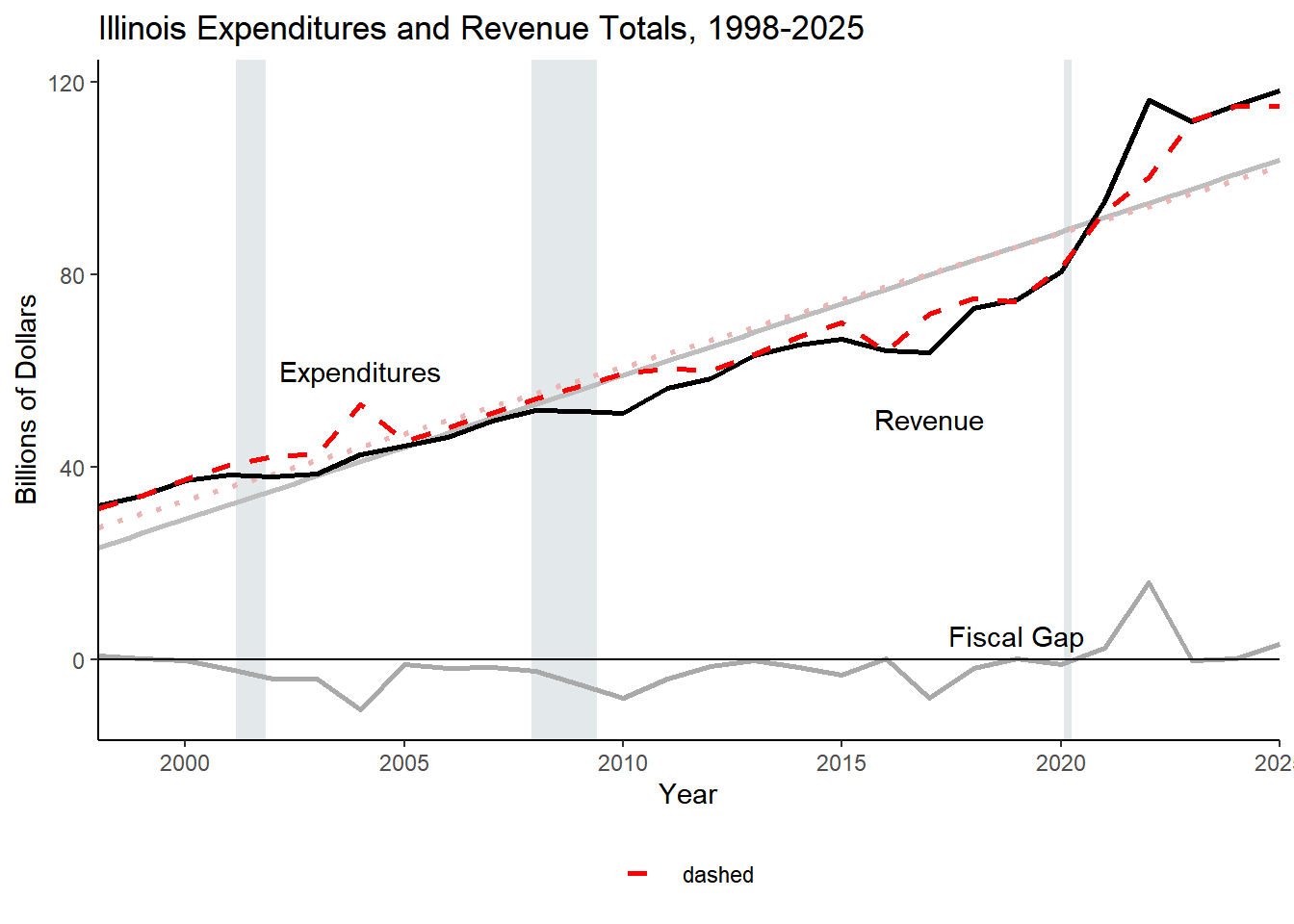
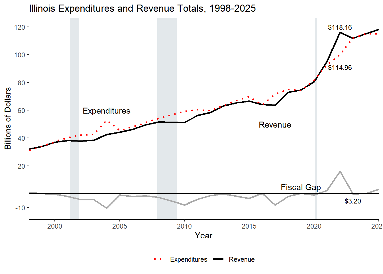
## Adjust x and y coordinates to move placement of text
annotation <- data.frame(
  x = c(2004, 2017, 2019),
  y = c(60, 50, 5),  
  label = c("Expenditures","Revenue", "Fiscal Gap")
)


annotation_nums <- data.frame(
  x = c(2022, 2022, 2023),
  y = c(91, 120, -5),  
  label = c(
   year_totals$Expenditures[year_totals$Year==current_year]/1000,
  year_totals$Revenue[year_totals$Year==current_year]/1000, 
  year_totals$`Fiscal Gap`[year_totals$Year==current_year]/1000)
)

## Dashed line versions for expenditures: 
fiscal_gap <-   
  ggplot(data = year_totals, aes(x=Year, y = Revenue/1000)) +
  geom_recessions(text = FALSE, update = recessions)+

  # geom_smooth adds regression line, graphed first so it appears behind line graph
  geom_smooth(aes(x = Year, y = Revenue/1000), color = "gray", alpha = 0.7, method = "lm", se = FALSE) + 
  #  scale_linetype_manual(values="dashed")+
  geom_smooth(aes(x = Year, y = Expenditures/1000), color ="rosybrown2", linetype = "dotted", method = "lm", se = FALSE, alpha = 0.7) +

  # line graph of revenue and expenditures
  geom_line(aes(x = Year, y = Revenue/1000), color = "Black", size=1) +
  geom_line(aes(x = Year, y = Expenditures/1000, linetype = "dashed"), color = "red", lwd=1) +
  geom_line(aes(x = Year, y = (`Fiscal Gap`/1000)), color = "darkgray", lwd = 1) +
    geom_hline(yintercept = 0) +

  geom_text(data = annotation, aes(x=x, y=y, label=label,
  parse = TRUE))+
  # labels
    theme_classic() +
    theme(legend.position = "bottom", legend.title = element_blank())+
    scale_linetype_manual(values = c("dashed", "dashed")) +
  scale_x_continuous(expand = c(0,0)) +

#  scale_y_continuous(labels = comma)+
  xlab("Year") + 
  ylab("Billions of Dollars")  +
  ggtitle(paste0("Illinois Expenditures and Revenue Totals, 1998-",current_year))

fiscal_gap

# annotation_billions <- data.frame(
#   x = c(2004, 2017, 2019),
#   y = c(60, 50, 5),  
#   label = c("Expenditures","Revenue", "Fiscal Gap"))


fiscal_gap2 <- ggplot(data = year_totals, aes(x=Year, y = Revenue/1000)) +
  geom_recessions(text = FALSE, update_recessions = recessions)+
  geom_line(aes(x = Year, y = Revenue/1000,  color = "Revenue"), lwd = 1, label = "Revenue") +
  geom_line(aes(x = Year, y = Expenditures/1000, color = "Expenditures"),  linetype = "dotted", lwd = 1, label = "Expenditures") +
  geom_line(aes(x = Year, y = (`Fiscal Gap`/1000)), color = "darkgray", lwd=1) +
  
  geom_text(data = annotation, aes(x=x, y=y, label=label)) + ## Word locations and text
  geom_text(data = annotation_nums, aes(x = x, y = y, label = scales::dollar(label, accuracy = 0.01L)), size = 3) +  ## Number locations and text
  theme_classic() +
  theme(legend.position = "bottom", legend.title = element_blank()) +
  scale_color_manual(values = c("Revenue" = "black", "Expenditures" = "red")) + 
  geom_hline(yintercept = 0) +

  scale_y_continuous(#labels = comma, 
                     limits = c(-12, 120), 
                     breaks = c(-10, 20, 40, 60, 80, 100, 120), 
                     minor_breaks = c(-10, 0, 10, 30, 50, 70, 90, 110))+
  scale_x_continuous(expand = c(0,0), 
                     limits = c(1998, current_year)
                     ) +
 # scale_color_manual(values = c("red" = "Expenditures", "black" = "Revenue")) + 

  xlab("Year") + 
  ylab("Billions of Dollars")  +
  ggtitle(paste0("Illinois Expenditures and Revenue Totals, 1998-",current_year))


fiscal_gap2

Expenditure and revenue amounts in billions of dollars:

Code

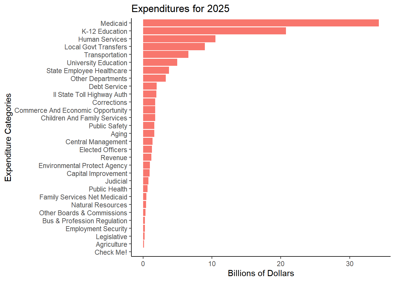
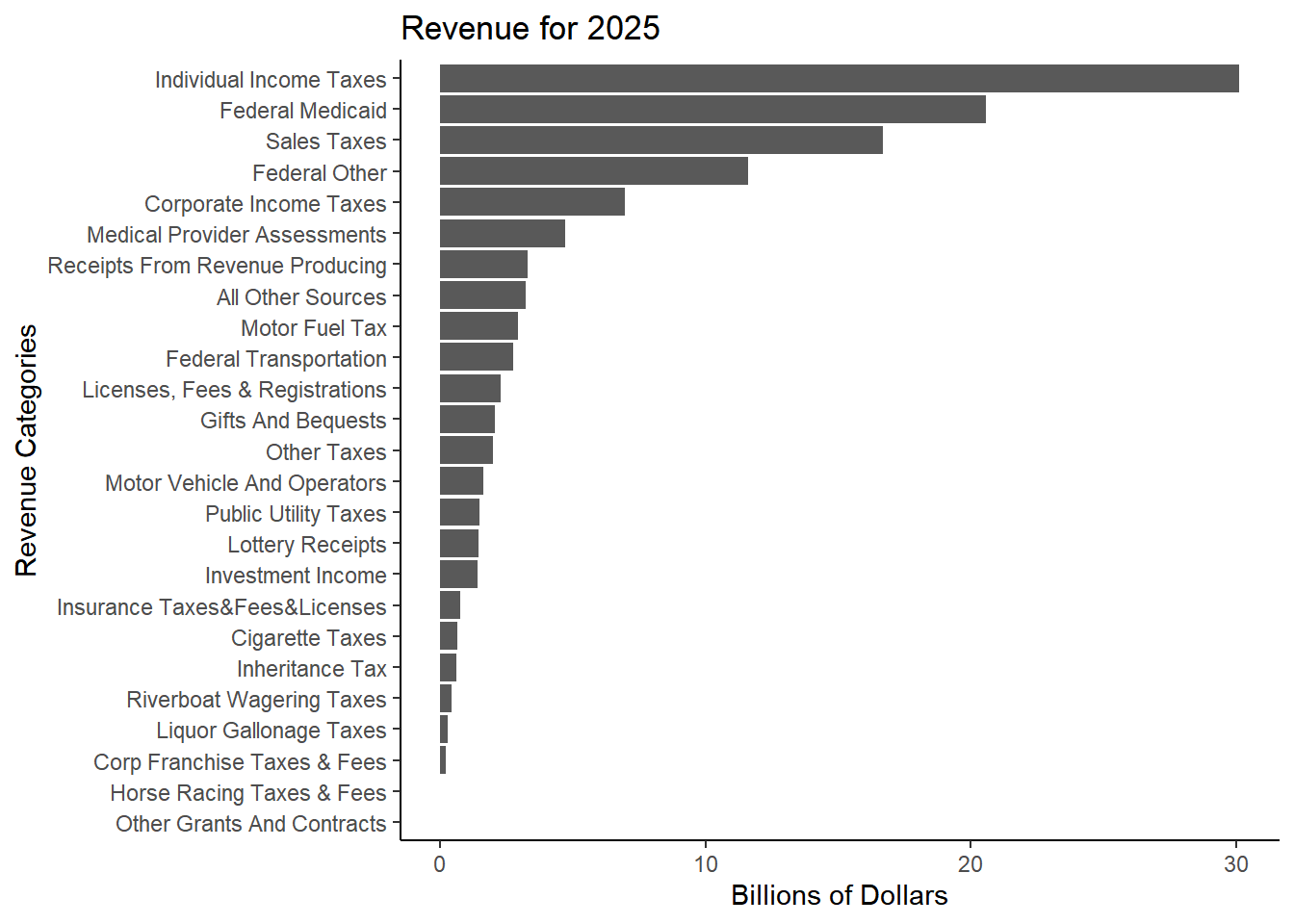
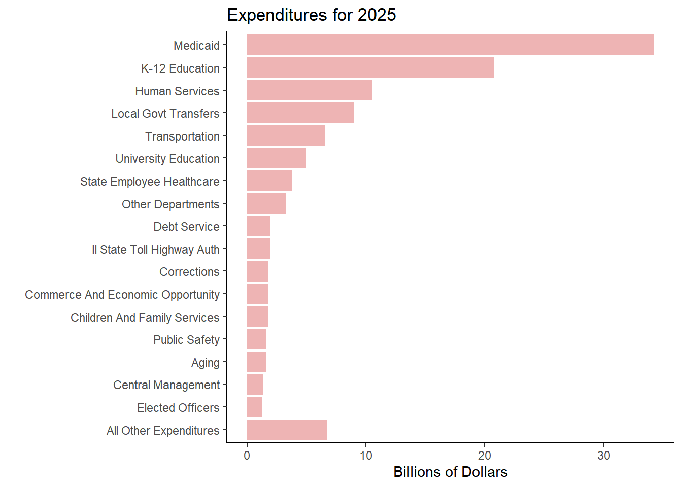
exp_long %>%
  filter(Year == current_year) %>%
  arrange(desc(`Dollars`)) %>%
  ggplot() + 
  geom_col(aes(x = fct_reorder(Category_name, `Dollars`), y = (`Dollars`/1000), fill = "red"))+ 
  coord_flip() +
      theme_classic()+
  theme(legend.position = "none") +
      labs(title = paste0("Expenditures for ", current_year))+    xlab("Expenditure Categories") +
  ylab("Billions of Dollars") 

rev_long %>%
  filter(Year == current_year) %>%
  arrange(desc(`Dollars`)) %>%
  ggplot() + 
  geom_col(aes(x = fct_reorder(Category_name, `Dollars`), y = (`Dollars`/1000)))+ 
  coord_flip() +
    theme_classic() +
    theme(legend.position = "none") +
      labs(title = paste0("Revenue for ", current_year))+
    xlab("Revenue Categories") +
  ylab("Billions of Dollars")

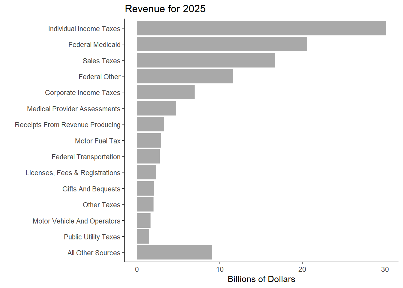
Expenditure and revenues when focusing on largest categories and combining others into “All Other Expenditures(Revenues)”:

Code

exp_long %>%
  filter( Year == current_year) %>%
  mutate(rank = rank(Dollars),
        Category_name = ifelse(rank > 13, Category_name, 'All Other Expenditures')) %>%
 # select(-c(Year, Dollars, rank)) %>%
  arrange(desc(Dollars)) %>%
  ggplot() + 
  geom_col(aes(x = fct_reorder(Category_name, `Dollars`), y = `Dollars`/1000), fill = "rosybrown2") + 
  coord_flip() +
      theme_classic() +
      labs(title = paste0("Expenditures for ", current_year))+    xlab("") +
  ylab("Billions of Dollars")

rev_long %>%
  filter( Year == current_year) %>%
  mutate(rank = rank(Dollars),
        Category_name = ifelse(rank > 10, Category_name, 'All Other Sources')) %>%
  arrange(desc(Dollars)) %>%
  ggplot() + 
  geom_col(aes(x = fct_reorder(Category_name, `Dollars`/1000), y = `Dollars`/1000), fill = "dark gray")+ 
  coord_flip() +
      theme_classic() +
      labs(title = paste0("Revenue for ", current_year)) +  
  xlab("") +
  ylab("Billions of Dollars")

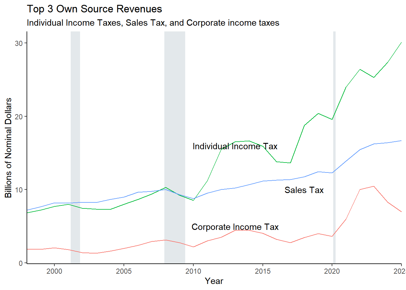
4.0.2 Top 3 Revenues

Code

annotation <- data.frame(
  x = c(2013, 2018, 2013),
  y = c(16, 10, 5),  
  label = c("Individual Income Tax", "Sales Tax", "Corporate Income Tax")
)

top3 <- rev_long  %>% 
  filter(Category == "02" | Category == "03" | Category == "06")

top3 <- ggplot(data = top3, aes(x=Year, y=Dollars/1000))+
      geom_recessions(text = FALSE, update = recessions)+
  geom_line(aes(x=Year, y=Dollars/1000, color = Category_name)) + 
  geom_text(data = annotation, aes(x=x, y=y, label=label)) +
  theme_classic() +
  scale_x_continuous(expand = c(0,0)) +
  scale_y_continuous(labels = comma) +
  scale_linetype_manual(values = c("dotted", "dashed", "solid")) +
  theme(legend.position = "none") +
  labs(title = "Top 3 Own Source Revenues", 
       subtitle = "Individual Income Taxes, Sales Tax, and Corporate income taxes",
       y = "Billions of Nominal Dollars") 
  
top3

Figure 4.5: Top 3 Revenue Sources (Own-Source Revenues only)

4.0.3 Own Source and Fed Transfers

Code

ownsource_rev <- rev_long %>%
  filter(!Category %in% c("57", "58", "59")) %>%
  group_by(Year) %>% 
  summarize(Dollars = sum(Dollars))

ownsource_rev
# ownsource_rev %>% 
#   ggplot()+geom_line(aes(x=Year, y=Dollars)) + 
#   labs(title = "Own Source Revenues", subtitle = "Total own source revenue", y = "Millions of Dollars")

Table 4.3: Own Source and Federal Revenue

Code

fed_rev <- ff_rev %>% 
  select(fy, rev_57, rev_58, rev_59) %>%
  mutate(fed_total = rev_57+rev_58+rev_59)


annotation <- data.frame(
  x = c(2013, 2015),
  y = c(50, 25),  
  label = c("Own Source Revenue", "Federal Revenue")
)

annotation_nums <- data.frame(
  x = c(2023, 2023),
  y = c(50, 25),  
  label = c("Own Source Revenue", "Federal Revenue")
)

ownsource_graph <- ggplot(ownsource_rev, aes(x=Year, y=Dollars/1000)) + 
  geom_recessions(text = FALSE, update_recessions = recessions)+
  geom_line(data = ownsource_rev, aes(x=Year, y=Dollars/1000), color = "Red") + 
  geom_line(data = fed_rev, aes(x=fy, y=fed_total/1000), color = "Black") + 
    geom_text(data = annotation, aes(x=x, y=y, label=label))+
    scale_y_continuous(labels = comma)+
  scale_x_continuous(expand = c(0,0)) + 
  theme(legend.position = "none") +

  theme_classic()+
  labs(title = "Own Source Revenue and Federal Revenue, 1998-2023", 
  y = "Billions of Dollars")
ownsource_graph

Code

# ggsave(plot = ownsource_graph, file = "Figure4.eps")

5 Change from Previous Year

Each year, you will need to update the CAGR formulas! Change the filter() year.

calc_cagr is a function created for calculating the CAGRs for different spans of time.

Code

exp_totals <- ff_exp %>% 
  rowwise() %>% 
  mutate(exp_TOTALS = sum(across(exp_402:exp_970), na.rm=TRUE))

rev_totals <- ff_rev %>%    
  rowwise() %>% 
  mutate(rev_TOTALS = sum(across(rev_02:rev_78), na.rm=TRUE))



rev_long <- pivot_longer(rev_totals, rev_02:rev_TOTALS, names_to = c("type","Category"), values_to = "Dollars", names_sep = "_") %>% 
  rename(Year = fy) %>%
  mutate(Category_name = case_when(
    Category == "02" ~ "INDIVIDUAL INCOME TAXES" ,
    Category == "03" ~ "CORPORATE INCOME TAXES" ,
    Category == "06" ~ "SALES TAXES" ,
    Category == "09" ~ "MOTOR FUEL TAX" ,
    Category == "12" ~ "PUBLIC UTILITY TAXES" ,
    Category == "15" ~ "CIGARETTE TAXES" ,
    Category == "18" ~ "LIQUOR GALLONAGE TAXES" ,
    Category == "21" ~ "INHERITANCE TAX" ,
    Category == "24" ~ "INSURANCE TAXES&FEES&LICENSES" ,
    Category == "27" ~ "CORP FRANCHISE TAXES & FEES" ,
    Category == "30" ~ "HORSE RACING TAXES & FEES",  # in Other
    Category == "31" ~ "MEDICAL PROVIDER ASSESSMENTS" ,
    Category == "32" ~ "GARNISHMENT-LEVIES" , # dropped
    Category == "33" ~  "LOTTERY RECEIPTS" ,
    Category == "35" ~  "OTHER TAXES" ,
    Category == "36" ~  "RECEIPTS FROM REVENUE PRODUCING", 
    Category == "39" ~  "LICENSES, FEES & REGISTRATIONS" ,
    Category == "42" ~  "MOTOR VEHICLE AND OPERATORS" ,
    Category == "45" ~  "STUDENT FEES-UNIVERSITIES",   # dropped
    Category == "48" ~  "RIVERBOAT WAGERING TAXES" ,
    Category == "51" ~  "RETIREMENT CONTRIBUTIONS" , # dropped
    Category == "54" ~ "GIFTS AND BEQUESTS", 
    Category == "57" ~  "FEDERAL OTHER" ,
    Category == "58" ~  "FEDERAL MEDICAID", 
    Category == "59" ~  "FEDERAL TRANSPORTATION" ,
    Category == "60" ~  "OTHER GRANTS AND CONTRACTS", #other
    Category == "63" ~  "INVESTMENT INCOME", # other
    Category == "66" ~ "PROCEEDS,INVESTMENT MATURITIES" , #dropped
    Category == "72" ~ "BOND ISSUE PROCEEDS",  #dropped
    Category == "75" ~  "INTER-AGENCY RECEIPTS ",  #dropped
    Category == "76" ~  "TRANSFER IN FROM OUT FUNDS",  #other
    Category == "78" ~  "ALL OTHER SOURCES" ,
    Category == "79" ~   "COOK COUNTY IGT", #dropped
    Category == "98" ~  "PRIOR YEAR REFUNDS", #dropped
    Category == "TOTALS" ~ "Total",
    T ~ "CHECK ME"
    
  ) ) %>% 
  select(-type, -Category) %>%  # drop extra columns type and Category number
  group_by(Year, Category_name) %>%
  summarise(Dollars= round(sum(Dollars, na.rm=TRUE), digits=2)) %>% 
  mutate(Category_name = str_to_title(Category_name))

# creates wide version of table where each revenue source is a column
revenue_wide2 <- rev_long %>% 
  pivot_wider(names_from = Category_name, 
              values_from = Dollars) %>%
  #  relocate("Other Revenue Sources **", .after = last_col()) %>%
  relocate("Total", .after =  last_col())

Code

exp_long <- pivot_longer(exp_totals, exp_402:exp_TOTALS , names_to = c("type", "Category"), values_to = "Dollars", names_sep = "_") %>%

  rename(Year = fy ) %>% 
  mutate(Category_name = 
           case_when(
             Category == "402" ~ "AGING" ,
             Category == "406" ~ "AGRICULTURE", 
             Category == "416" ~ "Central Management",
             Category == "418" ~ "CHILDREN AND FAMILY SERVICES", 
             Category == "420" ~ "Community Development",
             Category == "422" ~ "NATURAL RESOURCES" ,
             Category == "426" ~ "CORRECTIONS",
             Category == "427" ~ "EMPLOYMENT SECURITY" ,
             Category == "442" ~ "Human Rights" ,
             
             Category == "444" ~ "Human Services" ,
             Category == "445" ~ "IL Power Agency" ,
             Category == "452" ~ "Labor" ,
             Category == "458" ~ "State Lottery" ,
             
             Category == "478" ~ "HEALTHCARE & FAM SER NET OF MEDICAID", 
             Category == "482" ~ "PUBLIC HEALTH", 
             Category == "492" ~ "REVENUE", 
             Category == "494" ~ "Transportation" ,
             Category == "497" ~ "Veterans' Affairs" ,
             Category == "507" ~ "GOMB",

             Category == "532" ~ "ENVIRONMENTAL PROTECT AGENCY" ,
             Category == "557" ~ "Tollway" ,
             Category == "901" ~ "State Pension Contribution",
             Category == "903" ~ "Debt Service",
             Category == "904" ~ "State Employee Healthcare",
             Category == "910" ~ "LEGISLATIVE"  ,
             Category == "920" ~ "JUDICIAL" ,
             Category == "930" ~ "ELECTED OFFICERS" , 
             Category == "941" ~ "Public Safety" ,
             Category == "942" ~ "ECON DEVT & INFRASTRUCTURE" ,
             Category == "943" ~ "CENTRAL SERVICES",
             Category == "944" ~ "BUS & PROFESSION REGULATION" ,
             Category == "945" ~ "Medicaid" ,
             Category == "946" ~ "Capital Improvement" , 
             Category == "948" ~ "OTHER DEPARTMENTS" ,
             Category == "949" ~ "OTHER BOARDS & COMMISSIONS" ,
             Category == "959" ~ "K-12 Education" ,
             Category == "960" ~ "UNIVERSITY EDUCATION",
             Category == "970" ~ "Local Govt Revenue Sharing",
             Category == "TOTALS" ~ "Total",
             T ~ "CHECK ME" 
            #  T ~ "All Other Expenditures **")
           )) %>% 
    select(-type, -Category) %>% 

   # mutate(Category_name = ifelse(Dollars < 1, "Other Departments", Category_name)) |>

  group_by(Year, Category_name) %>% 
  summarise(Dollars = round(sum(Dollars, na.rm=TRUE), digits=2)) %>% 
  mutate(Category_name = str_to_title(Category_name))

expenditure_wide2 <- exp_long %>% 
  pivot_wider(names_from = Category_name, 
              values_from = Dollars) %>%
  relocate("Total", .after =  last_col())

Things to do when updating the code:

Each year, you need to increase the cagr value by 1. The value should be the (current year - 1998). For FY23, this is 2023-1998 = 25. So all cagr values that were 24 will be changed to 25.

Code

max_cagr_years = current_year-1998

# function for calculating the CAGR
calc_cagr <- function(df, n) {
  df <- df %>%
    arrange(Category_name, Year) %>%
    group_by(Category_name) %>%
    mutate(cagr = ((`Dollars` / lag(`Dollars`, n)) ^ (1 / n)) - 1,
           cagr = ifelse(is.na(cagr), 0, cagr)
)

  return(df)
}

cagr_calculations <- function(df){ # This works for one variable at a time
  
  df <- df
  
  cagr_max <- calc_cagr(df, max_cagr_years) %>% 
    summarize(cagr_max = round(sum(cagr*100, na.rm = TRUE), 2))

  # Update year in the filter() and summarize() commands to current year.
  cagr_10 <- calc_cagr(df, 10) %>% 
    filter(Year == current_year) %>%
    summarize(cagr_10 = case_when(Year == current_year ~ round(sum(cagr*100, na.rm = TRUE), 2)))

  cagr_5 <- calc_cagr(df, 5) %>% 
    filter(Year == current_year) %>%
    summarize(cagr_5 = case_when(Year == current_year ~ round(sum(cagr*100, na.rm = TRUE), 2)))

  cagr_3 <- calc_cagr(df, 3) %>% 
    filter(Year == current_year) %>%
    summarize(cagr_3 = case_when(Year == current_year ~ round(sum(cagr*100, na.rm = TRUE), 2)))

  cagr_2 <- calc_cagr(df, 2) %>% 
    filter(Year == current_year) %>%
    summarize(cagr_2 = case_when(Year == current_year ~ round(sum(cagr*100, na.rm = TRUE), 2)))

  cagr_1 <- calc_cagr(df, 1) %>% 
    filter(Year == current_year) %>%
    summarize(cagr_1 = case_when(Year == current_year ~ round(sum(cagr*100, na.rm = TRUE), 2)))
  
    # Combine all into one tibble
  result <- data.frame(cagr_max, cagr_10, cagr_5, cagr_3, cagr_2, cagr_1)
  return(result)
  }

Code

CAGR_expenditures_summary_tot <- cagr_calculations(exp_long)   |>
  select(-c(Category_name.1, Category_name.2, Category_name.3, Category_name.4, Category_name.5 )) %>% 
  rename("Expenditure Category" = Category_name, "1 Year CAGR" = cagr_1, "2 Year CAGR" = cagr_2, "3 Year CAGR" = cagr_3, "5 Year CAGR" = cagr_5, "10 Year CAGR" = cagr_10, "27 Year CAGR" = cagr_max )


totalrow <- which(grepl("Total", CAGR_expenditures_summary_tot$`Expenditure Category`))

CAGR_expenditures_summary_tot <- move_to_last(CAGR_expenditures_summary_tot, totalrow) 

lastrow = nrow(CAGR_expenditures_summary_tot)


CAGR_expenditures_summary_tot %>%   
  kbl(caption = "CAGR Calculations for All Expenditure Categories" , row.names=FALSE) %>% 
  kable_classic() %>%
  row_spec(lastrow, bold = T, color = "black", background = "gray")

Table 5.1: Expenditure Category CAGRs with Total CAGR (Ordered Alphabetically)

CAGR Calculations for All Expenditure Categories
Expenditure Category	27 Year CAGR	10 Year CAGR	5 Year CAGR	3 Year CAGR	2 Year CAGR	1 Year CAGR
Aging	7.81	4.73	9.00	11.75	8.97	6.25
Agriculture	2.07	5.95	11.84	12.20	19.22	16.12
Bus & Profession Regulation	2.09	-1.51	6.57	7.16	7.82	5.97
Capital Improvement	4.91	2.18	24.62	29.79	19.71	12.80
Central Management	4.48	4.54	3.19	6.33	1.04	-0.30
Check Me	0.00	0.00	0.00	0.00	0.00	0.00
Children And Family Services	1.11	4.59	7.18	11.83	5.36	-2.37
Community Development	5.08	5.95	23.35	8.38	8.71	9.95
Corrections	2.21	2.53	2.96	5.82	2.19	-2.64
Debt Service	5.32	-0.26	0.16	-0.78	0.29	-14.24
Elected Officers	4.24	4.65	7.45	-0.30	-6.72	6.68
Employment Security	1.35	1.77	1.94	-1.78	-1.97	-2.05
Environmental Protect Agency	4.39	4.43	6.61	14.87	26.77	12.40
Healthcare & Fam Ser Net Of Medicaid	5.39	0.84	5.89	7.40	4.54	0.72
Human Services	3.71	5.95	11.89	13.07	9.15	0.49
Judicial	3.84	3.93	4.66	5.81	1.75	-1.59
K-12 Education	4.97	5.33	4.53	2.13	-0.68	-4.33
Legislative	5.04	8.29	13.27	15.26	-0.33	-2.49
Local Govt Revenue Sharing	3.58	3.65	6.85	-4.57	-9.18	-6.88
Medicaid	7.08	7.30	8.95	6.10	2.76	2.33
Natural Resources	2.91	3.27	9.15	13.91	15.70	12.94
Other Boards & Commissions	5.01	3.58	10.90	12.94	3.86	1.05
Other Departments	8.04	3.91	6.91	7.57	-1.80	5.31
Public Health	5.44	5.22	3.77	-6.99	-6.29	-7.80
Public Safety	5.03	7.70	2.01	-1.52	-2.84	-24.64
Revenue	3.79	10.10	0.79	-13.67	-37.87	-13.28
State Employee Healthcare	6.26	4.36	4.76	7.78	11.95	18.97
Tollway	6.33	0.16	0.08	-2.89	0.82	-2.62
Transportation	4.55	3.77	9.98	12.83	11.37	11.06
University Education	2.91	2.61	4.10	4.33	3.07	-1.12
Total	4.94	5.10	7.09	4.73	1.33	-0.03

Code

CAGR_revenue_summary_tot <- cagr_calculations(rev_long) %>%   
  select(-c(Category_name.1, Category_name.2, Category_name.3, Category_name.4, Category_name.5 )) %>% 
  rename("Revenue Category" = Category_name, "1 Year CAGR" = cagr_1, "2 Year CAGR" = cagr_2, "3 Year CAGR" = cagr_3, "5 Year CAGR" = cagr_5, "10 Year CAGR" = cagr_10, "27 Year CAGR" = cagr_max )

CAGR_revenue_summary_tot <- move_to_last(CAGR_revenue_summary_tot, 1)

totalrow <- which(grepl("Total", CAGR_revenue_summary_tot$`Revenue Category`))

CAGR_revenue_summary_tot <- move_to_last(CAGR_revenue_summary_tot, totalrow)

lastrow = nrow(CAGR_revenue_summary_tot)

CAGR_revenue_summary_tot %>% 
  kbl(caption = "CAGR Calculations for All Revenue Sources (Ordered Alphabetical)", row.names = FALSE) %>% 
   kable_classic() %>%
    row_spec(lastrow, bold = T, color = "black", background = "gray")

Table 5.2: Revenue Category CAGRs with Total CAGR (Ordered Alphabetically)

CAGR Calculations for All Revenue Sources (Ordered Alphabetical)
Revenue Category	27 Year CAGR	10 Year CAGR	5 Year CAGR	3 Year CAGR	2 Year CAGR	1 Year CAGR
Cigarette Taxes	1.32	-2.61	-4.91	-7.71	-8.20	-6.58
Corp Franchise Taxes & Fees	1.92	-0.66	-1.29	-2.93	-6.40	-2.69
Corporate Income Taxes	5.01	5.54	13.84	-11.48	-18.56	-16.23
Federal Medicaid	6.97	6.97	8.26	2.62	0.93	-3.72
Federal Other	4.28	6.45	3.65	-15.71	3.30	10.68
Federal Transportation	4.50	3.04	8.97	14.34	13.86	16.11
Gifts And Bequests	10.50	11.33	17.40	3.35	-1.23	-16.34
Horse Racing Taxes & Fees	-6.10	1.56	2.36	-3.08	0.32	-0.64
Individual Income Taxes	5.64	6.59	8.98	4.44	9.10	10.03
Inheritance Tax	3.31	6.10	16.30	-0.03	9.51	-3.93
Insurance Taxes&Fees&Licenses	6.64	4.81	9.36	7.15	6.45	13.15
Investment Income	6.18	38.91	40.04	157.55	36.97	11.20
Licenses, Fees & Registrations	7.71	6.36	9.80	6.29	4.84	-3.69
Liquor Gallonage Taxes	6.38	0.68	0.02	-1.80	-2.12	-2.60
Lottery Receipts	2.10	1.49	4.77	1.66	-3.09	-8.88
Medical Provider Assessments	8.33	9.16	6.29	8.07	7.36	8.55
Motor Fuel Tax	3.08	8.61	4.96	5.33	7.22	4.67
Motor Vehicle And Operators	2.95	0.63	2.38	0.88	1.33	0.15
Other Grants And Contracts	2.70	29.93	24.22	165.59	79.20	113.69
Other Taxes	8.11	12.57	19.52	11.44	10.68	17.71
Public Utility Taxes	0.79	0.01	0.74	1.53	1.18	2.65
Receipts From Revenue Producing	5.74	4.50	8.61	11.24	12.65	9.05
Riverboat Wagering Taxes	2.57	-1.09	5.07	9.35	9.34	15.57
Sales Taxes	3.17	4.12	6.35	2.57	1.46	1.67
All Other Sources	6.40	5.71	11.91	7.53	-1.02	-1.16
Total	4.95	5.90	7.95	0.60	2.82	2.64

Code

first_year = as.numeric(1998)
n_year_change = as.numeric(current_year-1998)



revenue_change2 <- rev_long %>%
  filter(Year >= past_year | Year == first_year) %>%
  pivot_wider(names_from = Year , values_from = Dollars,   names_prefix = "Dollars_") %>%
  rename(    
    Dollars_current = Dollars_2025,
    Dollars_lastyear = Dollars_2024
    )|>
  mutate(
    "Current FY ($ billions)" = round(Dollars_current/1000, digits = 2),
    "Past FY ($ billions)" = round(Dollars_lastyear/1000, digits = 2),
        "FY 1994 ($ billions)" = round(Dollars_1998/1000, digits = 2),
    "1-Year Change" = percent((Dollars_current -Dollars_lastyear)/Dollars_lastyear, accuracy = .01)) |>
  left_join(CAGR_revenue_summary_tot, by = c("Category_name" = "Revenue Category")) %>% 
    arrange(-`Current FY ($ billions)`)%>%
    mutate(`27 Year CAGR` = percent(`27 Year CAGR`/100, accuracy=.01)) %>%

  rename(  
          "Revenue Category" = Category_name ) %>%
  select(-c( Dollars_1998, Dollars_current, Dollars_lastyear, `1 Year CAGR`:`10 Year CAGR`))


allother_row <- which(grepl("All Other", revenue_change2$`Revenue Category`))

revenue_change2 <- move_to_last(revenue_change2, allother_row) # Move "All Other" to 2nd to last row

totalrow <- which(grepl("Total", revenue_change2$`Revenue Category`))
revenue_change2 <- move_to_last(revenue_change2, totalrow) # Move "Total" to last row

lastrow = nrow(revenue_change2)

revenue_change2 %>%   
  filter(!is.na(`Revenue Category`)) %>%

  kbl(caption = "Table 1. Yearly Change in Revenue", row.names = FALSE) %>% 
   kable_classic() %>%
    row_spec(lastrow, bold = T, color = "black", background = "gray")

Table 5.3: Yearly Change in Revenues - All FF Categories, Ordered from Largest to Smallest Revenue Amount

Table 1. Yearly Change in Revenue
Revenue Category	Current FY ($ billions)	Past FY ($ billions)	FY 1994 ($ billions)	1-Year Change	27 Year CAGR
Individual Income Taxes	30.13	27.38	6.85	10.03%	5.64%
Federal Medicaid	20.58	21.38	3.34	-3.72%	6.97%
Sales Taxes	16.70	16.43	7.20	1.67%	3.17%
Federal Other	11.61	10.49	3.75	10.68%	4.28%
Corporate Income Taxes	6.95	8.30	1.86	-16.23%	5.01%
Medical Provider Assessments	4.71	4.34	0.54	8.55%	8.33%
Receipts From Revenue Producing	3.29	3.01	0.73	9.05%	5.74%
Motor Fuel Tax	2.95	2.82	1.30	4.67%	3.08%
Federal Transportation	2.74	2.36	0.84	16.11%	4.50%
Licenses, Fees & Registrations	2.26	2.35	0.30	-3.69%	7.71%
Gifts And Bequests	2.05	2.45	0.14	-16.34%	10.50%
Other Taxes	2.01	1.70	0.24	17.71%	8.11%
Motor Vehicle And Operators	1.64	1.64	0.75	0.15%	2.95%
Public Utility Taxes	1.48	1.44	1.19	2.65%	0.79%
Lottery Receipts	1.46	1.61	0.83	-8.88%	2.10%
Investment Income	1.40	1.26	0.28	11.20%	6.18%
Insurance Taxes&Fees&Licenses	0.75	0.66	0.13	13.15%	6.64%
Cigarette Taxes	0.66	0.71	0.46	-6.58%	1.32%
Inheritance Tax	0.60	0.63	0.25	-3.93%	3.31%
Riverboat Wagering Taxes	0.42	0.36	0.21	15.57%	2.57%
Liquor Gallonage Taxes	0.30	0.31	0.06	-2.60%	6.38%
Corp Franchise Taxes & Fees	0.21	0.21	0.12	-2.69%	1.92%
Horse Racing Taxes & Fees	0.01	0.01	0.04	-0.64%	-6.10%
Other Grants And Contracts	0.01	0.00	0.00	113.69%	2.70%
All Other Sources	3.24	3.28	0.61	-1.16%	6.40%
Total	118.16	115.13	32.03	2.64%	4.95%

Code

expenditure_change2 <- exp_long %>%
  group_by(Year, Category_name) |>
  summarize(Dollars = sum(Dollars, na.rm=TRUE)) |>
  ungroup() |>
  filter(Year >= past_year | Year == first_year) %>%
  pivot_wider(names_from = Year , values_from = Dollars,   names_prefix = "Dollars_") %>%
    rename(    
    Dollars_current = Dollars_2025,
    Dollars_lastyear = Dollars_2024
    )|>
  mutate(
    "FY 2025 ($ billions)" = round(Dollars_current/1000, digits = 2),
    "FY 2024 ($ billions)" = round(Dollars_lastyear/1000, digits = 2),
    "FY 1998 ($ billions)" = round(Dollars_1998/1000, digits = 2),
    "1-Year Change" = percent((Dollars_current -Dollars_lastyear)/Dollars_lastyear, accuracy = .01)) |>
  left_join(CAGR_expenditures_summary_tot, by = c("Category_name" = "Expenditure Category")) %>% 
  arrange(-`FY 2025 ($ billions)`)%>%
    mutate(`27 Year CAGR` = percent(`27 Year CAGR`/100, accuracy=.01)) %>%

  select(-c( Dollars_1998, Dollars_current, Dollars_lastyear, `1 Year CAGR`:`10 Year CAGR`)) %>%

  rename("Expenditure Category" = Category_name ) # |> filter(!is.na(`Expenditure Category`))


allother_row <- which(grepl("All Other", expenditure_change2$`Expenditure Category`))

expenditure_change2 <- move_to_last(expenditure_change2, allother_row) # Move "All Other" to 2nd to last row

totalrow <- which(grepl("Total", expenditure_change2$`Expenditure Category`))
expenditure_change2 <- move_to_last(expenditure_change2, totalrow) # Move "Total" to last row

lastrow = nrow(expenditure_change2)

expenditure_change2 %>% 
  kbl(row.names = FALSE) %>% 
  kable_classic() %>%
    row_spec(lastrow, bold = T, color = "black", background = "gray")

Table 5.4: Yearly Change in Expenditures - All FF Categories, Ordered from Largest to Smallest Expenditure Amount

Expenditure Category	FY 2025 ($ billions)	FY 2024 ($ billions)	FY 1998 ($ billions)	1-Year Change	27 Year CAGR
Medicaid	34.22	33.44	5.40	2.33%	7.08%
K-12 Education	20.77	21.71	5.60	-4.33%	4.97%
Human Services	10.52	10.47	3.93	0.49%	3.71%
Local Govt Revenue Sharing	8.99	9.66	3.48	-6.88%	3.58%
Transportation	6.57	5.91	1.98	11.06%	4.55%
University Education	4.96	5.02	2.28	-1.12%	2.91%
State Employee Healthcare	3.76	3.16	0.73	18.97%	6.26%
Other Departments	3.30	3.14	0.41	5.31%	8.04%
Debt Service	1.96	2.29	0.48	-14.24%	5.32%
Tollway	1.93	1.98	0.37	-2.62%	6.33%
Corrections	1.78	1.83	0.99	-2.64%	2.21%
Community Development	1.77	1.61	0.47	9.95%	5.08%
Children And Family Services	1.75	1.79	1.30	-2.37%	1.11%
Aging	1.64	1.54	0.22	6.25%	7.81%
Public Safety	1.64	2.18	0.44	-24.64%	5.03%
Central Management	1.39	1.40	0.43	-0.30%	4.48%
Elected Officers	1.28	1.20	0.42	6.68%	4.24%
Revenue	1.20	1.39	0.44	-13.28%	3.79%
Environmental Protect Agency	0.99	0.88	0.31	12.40%	4.39%
Capital Improvement	0.94	0.83	0.26	12.80%	4.91%
Judicial	0.78	0.79	0.28	-1.59%	3.84%
Public Health	0.67	0.73	0.16	-7.80%	5.44%
Healthcare & Fam Ser Net Of Medicaid	0.47	0.46	0.11	0.72%	5.39%
Natural Resources	0.43	0.38	0.20	12.94%	2.91%
Other Boards & Commissions	0.35	0.35	0.09	1.05%	5.01%
Bus & Profession Regulation	0.27	0.25	0.15	5.97%	2.09%
Employment Security	0.26	0.27	0.18	-2.05%	1.35%
Legislative	0.24	0.24	0.06	-2.49%	5.04%
Agriculture	0.13	0.11	0.07	16.12%	2.07%
Check Me	0.00	0.00	0.00	NA	0.00%
Total	114.96	115.00	31.24	-0.03%	4.94%

5.1 Summary Tables - Largest Categories

The 10 largest revenue sources and 15 largest expenditure sources remain separate categories and all other smaller sources/expenditures are combined into “All Other Revenues (Expenditures)”. These condensed tables are typically used in the Fiscal Futures articles. They were manually created in past years but this hopefully automates the process a bit until final formatting stages.

Table 5.5: Largest Revenue Categories with CAGRs

Code

n_categories <- 10+1 # (Top 10 and then Total )

rev_majorcats <- rev_long |> 
  filter(Year == current_year | Year == first_year
         ) |>
  arrange(desc(Dollars)) |>
  slice(1:n_categories)

rev_long_majorcats <- rev_long |>
  mutate(Category_name = ifelse(Category_name %in% rev_majorcats$Category_name, Category_name, "All Other Sources"),
         Category_name = ifelse(Category_name == "Total", "Total Revenue", Category_name)) |>
  group_by(Year, Category_name) |> 
  summarize(Dollars = sum(Dollars, na.rm=TRUE))


# creates wide version of table where each revenue source is a column
revenue_wide_majorcats <- rev_long_majorcats %>% 
  pivot_wider(names_from = Category_name, 
              values_from = Dollars) %>%
  relocate("All Other Sources", .after = last_col()) %>%
  relocate("Total Revenue", .after =  last_col())

Code

CAGR_revenue_majorcats_tot <- cagr_calculations(rev_long_majorcats) %>%   
  select(-c(Category_name.1, Category_name.2, Category_name.3, Category_name.4, Category_name.5 )) %>% 
  rename("Revenue Category" = Category_name, "1 Year CAGR" = cagr_1, "2 Year CAGR" = cagr_2, "3 Year CAGR" = cagr_3, "5 Year CAGR" = cagr_5, "10 Year CAGR" = cagr_10, "27 Year CAGR" = cagr_max )

allother_row <- which(grepl("All Other", CAGR_revenue_majorcats_tot$`Revenue Category`))

CAGR_revenue_majorcats_tot <- move_to_last(CAGR_revenue_majorcats_tot, allother_row) # Move "All Other" to 2nd to last row

totalrow <- which(grepl("Total", CAGR_revenue_majorcats_tot$`Revenue Category`))
CAGR_revenue_majorcats_tot <- move_to_last(CAGR_revenue_majorcats_tot, totalrow) # Move "Total" to last row

lastrow = nrow(CAGR_revenue_majorcats_tot)

CAGR_revenue_majorcats_tot %>% 
  kbl(caption = "CAGR Calculations for Largest Revenue Sources", row.names = FALSE) %>% 
  kable_classic() %>%
    row_spec(lastrow, bold = T, color = "black", background = "gray")

Table 5.6: Top 10 Revenue Sources with CAGRs

CAGR Calculations for Largest Revenue Sources
Revenue Category	27 Year CAGR	10 Year CAGR	5 Year CAGR	3 Year CAGR	2 Year CAGR	1 Year CAGR
Corporate Income Taxes	5.01	5.54	13.84	-11.48	-18.56	-16.23
Federal Medicaid	6.97	6.97	8.26	2.62	0.93	-3.72
Federal Other	4.28	6.45	3.65	-15.71	3.30	10.68
Federal Transportation	4.50	3.04	8.97	14.34	13.86	16.11
Individual Income Taxes	5.64	6.59	8.98	4.44	9.10	10.03
Lottery Receipts	2.10	1.49	4.77	1.66	-3.09	-8.88
Medical Provider Assessments	8.33	9.16	6.29	8.07	7.36	8.55
Motor Fuel Tax	3.08	8.61	4.96	5.33	7.22	4.67
Motor Vehicle And Operators	2.95	0.63	2.38	0.88	1.33	0.15
Public Utility Taxes	0.79	0.01	0.74	1.53	1.18	2.65
Receipts From Revenue Producing	5.74	4.50	8.61	11.24	12.65	9.05
Sales Taxes	3.17	4.12	6.35	2.57	1.46	1.67
All Other Sources	6.04	6.98	12.46	8.79	4.63	-0.14
Total Revenue	4.95	5.90	7.95	0.60	2.82	2.64

Code

###### Yearly change summary table for Top 10 Revenues #####
revenue_change_majorcats <- rev_long_majorcats %>%
  #select(-c(Category)) %>%
  filter(Year >= past_year |  Year == first_year) %>%
  pivot_wider(names_from = Year , values_from = Dollars,   names_prefix = "Dollars_") %>%
    rename(    
    Dollars_current = Dollars_2025,
    Dollars_lastyear = Dollars_2024
    )|>
  mutate(
    "Current FY ($ billions)" = round(Dollars_current/1000, digits = 2),
    "Previous FY ($ billions)" = round(Dollars_lastyear/1000, digits = 2),
    "FY 1998 ($ billions)" = round(Dollars_1998/1000, digits = 2),
    "1-Year Change" = percent((Dollars_current -Dollars_lastyear)/Dollars_lastyear, accuracy = .01),
  )  %>%
  left_join(CAGR_revenue_majorcats_tot, by = c("Category_name" = "Revenue Category")
            ) %>% 
  arrange(-`Current FY ($ billions)`)%>%
  mutate(`27 Year CAGR` = percent(`27 Year CAGR`/100, accuracy=.01)) %>%
  select(-c(Dollars_1998, Dollars_current, Dollars_lastyear, `1 Year CAGR`:`10 Year CAGR`
            )) %>%
  rename("Revenue Category" = Category_name )

allother_row <- which(grepl("All Other", revenue_change_majorcats$`Revenue Category`))

revenue_change_majorcats <- move_to_last(revenue_change_majorcats, allother_row) # Move "All Other" to 2nd to last row

totalrow <- which(grepl("Total", revenue_change_majorcats$`Revenue Category`))
revenue_change_majorcats <- move_to_last(revenue_change_majorcats, totalrow) # Move "Total" to last row

lastrow = nrow(revenue_change_majorcats)

revenue_change_majorcats%>% 
  kbl(caption = "Yearly Change in Revenue for Main Revenue Sources", row.names = FALSE, align = "l") %>% 
   kable_classic() %>%
    row_spec(lastrow, bold = T, color = "black", background = "gray")

Table 5.7: Top 10 Revenue Sources with CAGRs

Yearly Change in Revenue for Main Revenue Sources
Revenue Category	Current FY ($ billions)	Previous FY ($ billions)	FY 1998 ($ billions)	1-Year Change	27 Year CAGR
Individual Income Taxes	30.13	27.38	6.85	10.03%	5.64%
Federal Medicaid	20.58	21.38	3.34	-3.72%	6.97%
Sales Taxes	16.70	16.43	7.20	1.67%	3.17%
Federal Other	11.61	10.49	3.75	10.68%	4.28%
Corporate Income Taxes	6.95	8.30	1.86	-16.23%	5.01%
Medical Provider Assessments	4.71	4.34	0.54	8.55%	8.33%
Receipts From Revenue Producing	3.29	3.01	0.73	9.05%	5.74%
Motor Fuel Tax	2.95	2.82	1.30	4.67%	3.08%
Federal Transportation	2.74	2.36	0.84	16.11%	4.50%
Motor Vehicle And Operators	1.64	1.64	0.75	0.15%	2.95%
Public Utility Taxes	1.48	1.44	1.19	2.65%	0.79%
Lottery Receipts	1.46	1.61	0.83	-8.88%	2.10%
All Other Sources	13.92	13.94	2.86	-0.14%	6.04%
Total Revenue	118.16	115.13	32.03	2.64%	4.95%

Code

n_categories <- 9 + 1 # (Top 9 and then Total )

exp_majorcats <- exp_long |> 
  filter(Year == current_year | Year == first_year
         ) |>
  arrange(desc(Dollars)) |>
  slice(1:n_categories) # keep top 10 largest categories or categories larger than 2 billion for final table in report (not a set rule, changes each year depending what the focus of the report is or what is highlighted.)


exp_long_majorcats <- exp_long |>
  mutate(Category_name = ifelse(Category_name %in% exp_majorcats$Category_name, Category_name, "All Other Expenditures **"),
         Category_name = ifelse(Category_name == "Total", "Total Expenditures", Category_name)) |>
  group_by(Year, Category_name) |> 
  summarize(Dollars = sum(Dollars, na.rm=TRUE))

# expenditure_wide_majorcats <- exp_long_majorcats %>% 
#   pivot_wider(names_from = Category_name, 
#               values_from = Dollars) %>%
#   relocate("All Other Expenditures **", .after = last_col()) %>%
#   relocate("Total Expenditures", .after =  last_col())



# CAGR values for largest expenditure categories and combined All Other Expenditures


CAGR_expenditures_majorcats_tot <- cagr_calculations(exp_long_majorcats) |>
  select(-c(Category_name.1, Category_name.2, Category_name.3, Category_name.4, Category_name.5 )) %>% 
  rename("Expenditure Category" = Category_name, "1 Year CAGR" = cagr_1, "2 Year CAGR" = cagr_2, "3 Year CAGR" = cagr_3, "5 Year CAGR" = cagr_5, "10 Year CAGR" = cagr_10,"27 Year CAGR" = cagr_max )

allother_row <- which(grepl("Other", CAGR_expenditures_majorcats_tot$`Expenditure Category`))

CAGR_expenditures_majorcats_tot <- move_to_last(CAGR_expenditures_majorcats_tot, allother_row) # Move "All Other" to 2nd to last row

totalrow <- which(grepl("Total", CAGR_expenditures_majorcats_tot$`Expenditure Category`))
CAGR_expenditures_majorcats_tot <- move_to_last(CAGR_expenditures_majorcats_tot, totalrow) # Move "Total" to last row

lastrow = nrow(CAGR_expenditures_majorcats_tot)

CAGR_expenditures_majorcats_tot%>%   
  kbl(caption = "CAGR Calculations for Largest Expenditure Categories" , row.names=FALSE) %>% 
     kable_classic()  %>%
    row_spec(lastrow, bold = T, color = "black", background = "gray")
# Yearly change for Top n largest expenditure categories
expenditure_change_majorcats <- exp_long_majorcats %>%
  filter(Year >= past_year |
           Year == first_year) %>%
  pivot_wider(names_from = Year , values_from = Dollars,   names_prefix = "Dollars_") %>%   
  rename(    
    Dollars_current = Dollars_2025,
    Dollars_lastyear = Dollars_2024
    )|>
  mutate("Current FY ($ Billions)" = round(Dollars_current/1000, digits = 2),
         "Previous FY ($ Billions)" = round(Dollars_lastyear/1000, digits = 2),
         "FY 1998 ($ Billions)" = round(Dollars_1998/1000, digits = 2),
         "1-Year Change" = percent((Dollars_current -Dollars_lastyear)/Dollars_lastyear, accuracy = .01),
         )  %>%
 left_join(CAGR_expenditures_majorcats_tot, by = c("Category_name" = "Expenditure Category")) %>% 
  arrange(-`Current FY ($ Billions)`)%>%
  mutate(`27 Year CAGR` = percent(`27 Year CAGR`/100, accuracy=.01)) %>%
  select(-c(Dollars_1998, Dollars_current, Dollars_lastyear, `1 Year CAGR`:`10 Year CAGR`
            )) %>%
  rename(
   # "1-Year Change" = `1 Year CAGR`,
    "27 Year Change" = `27 Year CAGR`, 
          "Expenditure Category" = Category_name )

allother_row <- which(grepl("All Other", expenditure_change_majorcats$`Expenditure Category`))

expenditure_change_majorcats <- move_to_last(expenditure_change_majorcats, allother_row) # Move "All Other" to 2nd to last row

totalrow <- which(grepl("Total", expenditure_change_majorcats$`Expenditure Category`))
expenditure_change_majorcats <- move_to_last(expenditure_change_majorcats, totalrow) # Move "Total" to last row

lastrow = nrow(expenditure_change_majorcats)

expenditure_change_majorcats %>% 
  kbl(caption = "Yearly Change in Expenditures", row.names = FALSE, align = "l") %>% 
  kable_classic() %>%
    row_spec(lastrow, bold = T, color = "black", background = "gray")

Table 5.8: Largest Expenditure Categories with CAGRs

CAGR Calculations for Largest Expenditure Categories
Expenditure Category	27 Year CAGR	10 Year CAGR	5 Year CAGR	3 Year CAGR	2 Year CAGR	1 Year CAGR
Children And Family Services	1.11	4.59	7.18	11.83	5.36	-2.37
Corrections	2.21	2.53	2.96	5.82	2.19	-2.64
Debt Service	5.32	-0.26	0.16	-0.78	0.29	-14.24
Human Services	3.71	5.95	11.89	13.07	9.15	0.49
K-12 Education	4.97	5.33	4.53	2.13	-0.68	-4.33
Local Govt Revenue Sharing	3.58	3.65	6.85	-4.57	-9.18	-6.88
Medicaid	7.08	7.30	8.95	6.10	2.76	2.33
State Employee Healthcare	6.26	4.36	4.76	7.78	11.95	18.97
Transportation	4.55	3.77	9.98	12.83	11.37	11.06
University Education	2.91	2.61	4.10	4.33	3.07	-1.12
All Other Expenditures **	4.77	4.16	6.39	3.12	-2.30	-1.31
Other Departments	8.04	3.91	6.91	7.57	-1.80	5.31
Total Expenditures	4.94	5.10	7.09	4.73	1.33	-0.03

Yearly Change in Expenditures
Expenditure Category	Current FY ($ Billions)	Previous FY ($ Billions)	FY 1998 ($ Billions)	1-Year Change	27 Year Change
Medicaid	34.22	33.44	5.40	2.33%	7.08%
K-12 Education	20.77	21.71	5.60	-4.33%	4.97%
Human Services	10.52	10.47	3.93	0.49%	3.71%
Local Govt Revenue Sharing	8.99	9.66	3.48	-6.88%	3.58%
Transportation	6.57	5.91	1.98	11.06%	4.55%
University Education	4.96	5.02	2.28	-1.12%	2.91%
State Employee Healthcare	3.76	3.16	0.73	18.97%	6.26%
Other Departments	3.30	3.14	0.41	5.31%	8.04%
Debt Service	1.96	2.29	0.48	-14.24%	5.32%
Corrections	1.78	1.83	0.99	-2.64%	2.21%
Children And Family Services	1.75	1.79	1.30	-2.37%	1.11%
All Other Expenditures **	16.38	16.60	4.66	-1.31%	4.77%
Total Expenditures	114.96	115.00	31.24	-0.03%	4.94%

Export summary file with Totals

Code

#install.packages("openxlsx")
library(openxlsx)

#aggregated_totals_majorcats = rbind(rev_long, exp_long)

todaysdate = Sys.Date()
dataset_names <- list(#'Aggregate Revenues' = revenue_wide2, 
                      #'Aggregate Expenditures' = expenditure_wide2, 

                      
                      'Table 1' = revenue_change_majorcats, #Top categories with yearly change, 23 yr cagr
                      'Table 2' = expenditure_change_majorcats,
                      
                      'Appendix 1' = revenue_change2,
                      'Appendix 2' = expenditure_change2,
                      
                      'CAGR Rev-MajorCats' = CAGR_revenue_majorcats_tot, # Categories Match Table 1 in paper
                      'CAGR Exp-MajorCats' = CAGR_expenditures_majorcats_tot,  
                                            
                      'Fiscal Gap' = year_totals,    # Total Revenue, Expenditure, and Fiscal gap per year
                      
                      'aggregated_totals_long' = aggregated_totals_long#, # all data in long format. Good for creating pivot tables in Excel
                      
                   #   'aggregated_fewercategories' = aggregated_totals_majorcats # combines categories that have small amounts into "All Other" category
                      )

# no pension categories included as separate cateogry (except for specific pension repayments that happened in some years.) 
# pension costs are included with K-12 education, university education, etc
write.xlsx(dataset_names, file = paste0("data/FY", current_year, " Files/summary_file_FY", current_year,"_pensionsdissolved_", todaysdate, ".xlsx"))

Saves main items in one excel file named summary_file.xlsx. Delete eval=FALSE to run on local computer.

# Pension Costs Included within Department Expenditures {#sec-all-code-pensionchange} In previous reports, a expenditure category was created to represent all Pension spending. It was created by removing pension expenditures out of the agencies that that had the expenses in order to highlight the amount that was spent on pensions. As of the FY2024 report, pension expenditures will remain in the agency that has the pension expenses to better represent the total cost of providing a service to the public. However, we thought that readers also might be interested in total pension spending during current and past years. We have added a separate table showing this information but emphasize that pension spending is already incorporated in other spending categories and should not be added to the total shown in Table 1 of the report. ```{r setup, warning=FALSE, message=FALSE} knitr::opts_chunk$set(echo = TRUE, warning = FALSE, message = FALSE) library(tidyverse) library(formatR) library(lubridate) library(scales) library(kableExtra) library(ggplot2) library(readxl) library(janitor) #devtools::install_github("CMAP-REPOS/cmapplot") library(cmapplot) move_to_last <- function(df, n) df[c(setdiff(seq_len(nrow(df)), n), n), ] current_year <- 2025 # fiscal year, not calendar year past_year=current_year-1 rev_temp <- read_csv(paste0("data/FY", current_year, " Files/rev_temp.csv")) exp_temp <- read_csv(paste0("data/FY", current_year, " Files/exp_temp.csv")) ``` ```{r include=FALSE} update_recessions <- function(url = NULL, quietly = FALSE){ # Use default URL if user does not override if (is_null(url) | missing(url)) { url <- "https://data.nber.org/data/cycles/business_cycle_dates.json" } # locally bind variable names start_char <- end_char <- start_date <- end_date <- ongoing <- index <- peak <- trough <- NULL return( # attempt to download and format recessions table tryCatch({ recessions <- jsonlite::fromJSON(url) %>% # drop first row trough dplyr::slice(-1) %>% # convert peaks and troughs... dplyr::mutate( # ...to R dates start_date = as.Date(peak), end_date = as.Date(trough), # ... and clean char strings start_char = format(start_date, "%b %Y"), end_char = format(end_date, "%b %Y")) %>% # confirm ascending and create row number dplyr::arrange(start_date) %>% mutate(index = row_number()) %>% mutate( # Flag unfinished recessions ongoing = case_when( is.na(end_date) & index == max(.$index) ~ T, TRUE ~ F), # set ongoing recession to arbitrary future date end_date = case_when( ongoing ~ as.Date("2200-01-01"), TRUE ~ end_date), # mark ongoing recession in char field end_char = case_when( ongoing ~ "Ongoing", TRUE ~ end_char) ) %>% # clean up select(start_char, end_char, start_date, end_date, ongoing) if (!quietly) {message("Successfully fetched from NBER")} # Return recessions recessions }, error = function(cond){ if (!quietly) message("WARNING: Fetch or processing failed. `NULL` returned.") return(NULL) } ) ) } #recess_table <- list(build_recessions(update)) recessions <- update_recessions() ``` ## Modify Expenditure File ### Tax refunds For more details on refund items, see @sec-taxrefunds. Aggregate expenditures: Code refunds to match the rev_type codes (02=income taxes, 03=corporate income taxes, 06=sales tax, 09=motor fuel tax, 24=insurance taxes and fees, 35 = all other tax refunds). Ideally the money going in and out of the funds used for refunds would be approximately equal. If equal, would drop from Fiscal Futures analysis so that Revenue reflects the amount of money the state gets to keep (and the local portion that becomes the local govt transfer) ```{r} # What we want: To exclude refunds as expenditures from our expenditure totals. # Exclude funds that hold refund funds from both revenue and expenditure sides # Revenue neutral unless budget tricks are occurring # still want to examine refunds over time to compare to past years calculations tax_refund_long <- exp_temp %>% # filter out only refund objects # keeps these objects which represent revenue, insurance, treasurer,and financial and professional reg tax refunds filter(fund != "0401" & # fund != "0401" # removes State Trust Funds (object == "9900" | object=="9910"|object=="9921"|object=="9923"|object=="9925")) %>% # add revenue category numbers mutate(refund = case_when( object == "9900" ~ "FY23_Rebates", # part of COVID relief fund=="0278" & sequence == "00" ~ "02", # for income tax refund fund=="0278" & sequence == "01" ~ "03", # tax administration and enforcement and tax operations become corporate income tax refund fund == "0278" & sequence == "02" ~ "02", object=="9921" ~ "21", # inheritance tax and estate tax refund appropriation object=="9923" ~ "09", # motor fuel tax refunds obj_seq_type == "99250055" ~ "06", # sales tax refund fund=="0378" & object=="9925" ~ "24", # insurance privilege tax refund (fund=="0001" & object=="9925") | (object=="9925" & fund == "0384" & fy == 2023) ~ "35", # all other taxes T ~ "CHECK")) # if none of the items above apply to the observations, then code them as CHECK exp_temp <- left_join(exp_temp, tax_refund_long) %>% mutate(refund = ifelse(is.na(refund),"not refund", as.character(refund))) ``` ```{r} #| label: fig-tax-refunds #| fig-cap: Tax Refunds #| column: margin tax_refund <- tax_refund_long %>% group_by(refund, fy)%>% summarize(refund_amount = sum(expenditure, na.rm = TRUE)/1000000) %>% pivot_wider(names_from = refund, values_from = refund_amount, names_prefix = "ref_") %>% mutate_all(~replace_na(.,0)) %>% arrange(fy) tax_refund %>% pivot_longer(c(ref_02:ref_35, ref_FY23_Rebates), names_to = "Refund Type", values_to = "Amount") %>% ggplot()+ theme_classic()+ geom_line(aes(x=fy,y=Amount, group = `Refund Type`, color = `Refund Type`))+ labs(title = "Refund Types", caption = "Refunds are excluded from Expenditure totals and instead subtracted from Revenue totals") + labs(title = "Tax refunds", caption = "Rev_type codes: 02=income taxes, 03=corporate income taxes, 06=sales tax, 09=motor fuel tax, 24=insurance taxes and fees, 35 = all other tax refunds." ) # remove the items we recoded in tax_refund_long # exp_temp <- exp_temp %>% filter(refund == "not refund") ``` For FY23, the one-time abatement, object 9900, is included as an expenditure item within the Department of Revenue. ```{r} # manually adds the abatements as expenditure item and keeps on expenditure side. # otherwise ignored since it is in fund 0278 and exp_temp <- exp_temp %>% mutate(in_ff = ifelse(object == 9900, 1, in_ff)) ``` ### Pension Expenditures State pension contributions for TRS and SURS are largely captured with object=4431. **(State payments into pension fund).** State payments to the following pension systems: - Teachers Retirement System (TRS) Agency 493 --> K-12 Education (Group = 959) - New POB bond in 2019: Accelerated Bond Fund paid benefits in advance as lump sum - State Employee Retirement System (SERS) Agency 589 --> SERS Agency 589 - _Note: Object 4431 does not have SERS expenditures in it. Those are only in object 116X objects_ - State University Retirement System (SURS) Agency 693 --> University Education (Group = 960) - Judges Retirement System (JRS) Agency 275 --> Judicial (Group = 920) - General Assembly Retirement System (GARS) --> Legislative (Group 910) There are also "Other Post-Employment Benefits" (OPEBs). Expenditure object 4430 is for retirement benefits. While it is good to know the overall cost of pensions for the state, if you want to know the true cost of providing services, pension and other benefit costs should be included in the department that is paying employees to provide those services. > Change in pension coding in chunk below: ```{r fig-pensions, fig.cap="Pensions"} exp_temp <- exp_temp %>% arrange(fund) %>% mutate(pension = case_when( ## Commented out line below: (object=="4431") ~ 1, # 4431 = easy to find pension payments INTO fund (object=="1298" & # Purchase of Investments, Normally excluded (fy==2010 | fy==2011) & (fund=="0477" | fund=="0479" | fund=="0481")) ~ 3, #judges retirement OUT of fund # state borrowed money from pension funds to pay for core services during 2010 and 2011. # used to fill budget gap and push problems to the future. fund == "0319" ~ 4, # pension stabilization fund TRUE ~ 0) ) ``` ```{r fig-pensions-POB, fig.cap="Pension Expenditures"} # special accounting of pension obligation bond (POB)-funded contributions to JRS, SERS, GARS, TRS exp_temp <- exp_temp %>% # change object for 2010 and 2011, retirement expenditures were bond proceeds and would have been excluded mutate(object = ifelse((pension > 0 & in_ff == "0"), "4431", object)) %>% # changes weird teacher & judge retirement system pensions object to normal pension object 4431 mutate(pension = ifelse(pension > 0 & in_ff == "0", 6, pension)) %>% # coded as 6 if it was supposed to be excluded. mutate(in_ff = ifelse(pension > 0, "1", in_ff)) # # all other pensions objects codes get agency code 901 for State Pension Contributions # exp_temp <- exp_temp %>% # mutate(agency = ifelse(pension > 0, "901", as.character(agency)), # agency_name = ifelse(agency == "901", "State Pension Contributions", as.character(agency_name))) ``` Can also be thought of past commitments vs current contributions. - Where past commitments in the form of pension benefits paid out. **Current Employees vs Retired Employees** Current Employees: - Group Insurance Benefits Retired Employees: - Deferred Compensation - Medicare Retirees and Survivors of State of Illinois Employees Group Insurance Program (SEGIP) - Part of Medicare ```{r} exp_temp|> filter(fy==2024) |> filter((appr_org=="01" | appr_org == "65" | appr_org=="88") & (object=="4900" | object=="4400") )|> group_by(agency, agency_name) |> # separates CHIP from health and human services and saves it as Medicaid summarize(expenditure = sum(expenditure)) ``` Drop all cash transfers between funds, statutory transfers, and purchases of investments from expenditure data. ```{r drop-transfers} transfers_drop <- exp_temp %>% filter( agency == "799" | # statutory transfers object == "1993" | # interfund cash transfers object == "1298") # purchase of investments transfers_drop # items being dropped, # always check to make sure you aren't accidentally dropping something of interest. exp_temp <- anti_join(exp_temp, transfers_drop) ``` ### State employee healthcare costs > Commented out line of code that seperates healthcare costs. This should keep healthcare costs in the agency, similar to the change that was made for pensions. Also not grouping the agencies below into "Other Departments" until final steps of aggregation. Smallest agencies will be combined into Other Departments for final summary tables. agency=="507"| agency=="442" | agency=="445" | agency=="452" |agency=="458" | agency=="497" ~ "948", # other departments When healthcare costs are not manually separated into their own category, it looks like the costs shift to many of the smaller departments, such as: - GOMB (507) - Human Rights (442) - Illinois Power Agency (445) - Labor (452) - State Lottery (458) - Veteran's Affairs (497) ```{r} #| label: examine-bureau-of-benefits-expenditures #| include: false exp_temp |> filter(org_name == "BUREAU OF BENEFITS") |> group_by(fy, agency) |> summarize(expenditure = sum(expenditure) ) |> pivot_wider(names_from = "fy", values_from = "expenditure") exp_temp |> filter(org_name == "BUREAU OF BENEFITS") |> group_by(fy, agency) |> summarize(expenditure = sum(expenditure) ) |> ggplot() + geom_line(aes(x=fy, y=expenditure, group= agency, color = agency)) + scale_y_continuous(labels = scales::dollar) + labs(title="Bureau of Benefits Expenditures") exp_temp |> filter(org_name == "BUREAU OF BENEFITS") |> group_by(fy, object) |> summarize(expenditure = sum(expenditure) ) |> ggplot() + geom_line(aes(x=fy, y=expenditure, group= object, color = object)) + scale_y_continuous(labels = scales::dollar) + labs(title="Bureau of Benefits Expenditures") ``` ```{r} #| label: employee-healthcare #if observation is a group insurance contribution, then the expenditure amount is set to $0 (essentially dropped from analysis) # pretend eehc is named group_insurance_contribution or something like that # eehc coded as zero implies that it is group insurance # if eehc=0, then expenditures are coded as zero for group insurance to avoid double counting costs exp_temp <- exp_temp %>% mutate(eehc = ifelse( # group insurance contributions for 1998-2005 and 2013-present fund == "0001" & (object == "1180" | object =="1900") & agency == "416" & appr_org=="20", 0, 1) )%>% mutate(eehc = ifelse( # group insurance contributions for 2006-2012 fund == "0001" & object == "1180" & agency == "478" & appr_org=="80", 0, eehc) )%>% # group insurance contributions from road fund # coded with 1900 for some reason?? mutate(eehc = ifelse( fund == "0011" & object == "1900" & agency == "416" & appr_org=="20", 0, eehc) ) %>% mutate(expenditure = ifelse(eehc=="0", 0, expenditure)) %>% mutate(agency = case_when( ## turns specific items into State Employee Healthcare (agency=904) fund=="0907" & (agency=="416" & appr_org=="20") ~ "904", # central management Bureau of benefits using health insurance reserve fund=="0907" & (agency=="478" & appr_org=="80") ~ "904", # agency = 478: healthcare & family services using health insurance reserve - stopped using this in 2012 TRUE ~ as.character(agency))) %>% mutate(agency_name = ifelse( agency == "904", "STATE EMPLOYEE HEALTHCARE", as.character(agency_name)), in_ff = ifelse(agency == "904", 1, in_ff), group = ifelse(agency == "904", "904", as.character(agency))) # creates group variable # Default group = agency number healthcare_costs <- exp_temp %>% filter(group == "904") ``` ```{r transfers-to-local} exp_temp <- exp_temp %>% mutate( agency = case_when(fund=="0515" & object=="4470" & type=="08" ~ "971", # income tax to local governments fund=="0515" & object=="4491" & type=="08" & sequence=="00" ~ "971", # object is shared revenue payments fund=="0802" & object=="4491" ~ "972", #pprt transfer fund=="0515" & object=="4491" & type=="08" & sequence=="01" ~ "976", #gst to local fund=="0627" & object=="4472"~ "976" , # public transportation fund but no observations exist fund=="0648" & object=="4472" ~ "976", # downstate public transportation, but doesn't exist fund=="0515" & object=="4470" & type=="00" ~ "976", # object 4470 is grants to local governments object=="4491" & (fund=="0188"|fund=="0189") ~ "976", fund=="0187" & object=="4470" ~ "976", fund=="0186" & object=="4470" ~ "976", object=="4491" & (fund=="0413"|fund=="0414"|fund=="0415") ~ "975", #mft to local fund == "0952"~ "975", # Added Sept 29 2022 AWM. Transportation Renewal MFT TRUE ~ as.character(agency)), agency_name = case_when(agency == "971"~ "INCOME TAX 1/10 TO LOCAL", agency == "972" ~ "PPRT TRANSFER TO LOCAL", agency == "975" ~ "MFT TO LOCAL", agency == "976" ~ "GST TO LOCAL", TRUE~as.character(agency_name)), group = ifelse(agency>"970" & agency < "977", as.character(agency), as.character(group))) ``` ```{r fig-drop-local-transfers, fig.cap="Drop Transfers from State to Local Governments"} transfers_long <- exp_temp %>% filter(group == "971" |group == "972" | group == "975" | group == "976") transfers <- transfers_long %>% group_by(fy, group ) %>% summarize(sum_expenditure = sum(expenditure)/1000000) %>% pivot_wider(names_from = "group", values_from = "sum_expenditure", names_prefix = "exp_" ) exp_temp <- anti_join(exp_temp, transfers_long) dropped_inff_0 <- exp_temp %>% filter(in_ff == 0) exp_temp <- exp_temp %>% filter(in_ff == 1) # drops in_ff = 0 funds AFTER dealing with net-revenue above ``` ```{r debt-service} debt_drop <- exp_temp %>% filter(object == "8841" | object == "8811") # escrow OR principle #debt_drop %>% group_by(fy) %>% summarize(sum = sum(expenditure)) %>% arrange(-fy) debt_keep <- exp_temp %>% filter(fund != "0455" & (object == "8813" | object == "8800" )) # examine the debt costs we want to include #debt_keep %>% group_by(fy) %>% summarize(sum = sum(expenditure)) %>% arrange(-fy) exp_temp <- anti_join(exp_temp, debt_drop) exp_temp <- anti_join(exp_temp, debt_keep) debt_keep <- debt_keep %>% mutate( agency = ifelse(fund != "0455" & (object == "8813" | object == "8800"), "903", as.character(agency)), group = ifelse(fund != "0455" & (object == "8813" | object == "8800"), "903", as.character(group)), in_ff = ifelse(group == "903", 1, as.character(in_ff))) debt_keep_yearly <- debt_keep %>% group_by(fy, group) %>% summarize(debt_cost = sum(expenditure,na.rm=TRUE)/1000000) %>% select(-group) ``` ### Add Other Fiscal Future group codes ```{r group-codes} exp_temp <- exp_temp %>% #mutate(agency = as.numeric(agency) ) %>% # arrange(agency)%>% mutate( group = case_when( agency>"100"& agency<"200" ~ "910", # legislative agency == "528" | (agency>"200" & agency<"300") ~ "920", # judicial ###################################################### # Not used if we are not separating pension costs!! # pension > 0 ~ "901", # pensions ## New CODE: April 23rd, 2025: agency == "593" ~ "959", # TRS becomes part of K-12 costs agency == "594" ~ "959", # TRS agency == "589" ~ "948", # SERS becomes part of "Other Agencies" agency == "693" ~ "960", # SURS becomes part of group 960 agency == "275" ~ "920", # JRS becomes part of group 920 agency == "131" ~ "910", # GARS becomes part of Group 910 ###################################################### (agency>"309" & agency<"400") ~ "930", # elected officers: Governor, lt gov, attorney general, sec. of state, comptroller, treasurer agency == "586" ~ "959", # create new K-12 group agency=="402" | agency=="418" | agency=="478" | agency=="444" | agency=="482" ~ as.character(agency), # aging, CFS, HFS, human services, public health T ~ as.character(group)) ) %>% mutate(group = case_when( agency=="478" & (appr_org=="01" | appr_org == "65" | appr_org=="88") & (object=="4900" | object=="4400") ~ "945", # separates CHIP from health and human services and saves it as Medicaid agency == "586" & fund == "0355" ~ "945", # 586 (Board of Edu) has special education which is part of medicaid # OLD CODE: agency == "586" & appr_org == "18" ~ "945", # Spec. Edu Medicaid Matching agency=="425" | agency=="466" | agency=="546" | agency=="569" | agency=="578" | agency=="583" | agency=="591" | agency=="592" | agency=="493" | agency=="588" ~ "941", # public safety & Corrections agency=="420" | agency=="494" | agency=="406" | agency=="557" ~ as.character(agency), # econ devt & infra, tollway agency=="511" | agency=="554" | agency=="574" | agency=="598" ~ "946", # Capital improvement agency=="422" | agency=="532" ~ as.character(agency), # environment & nat. resources agency=="440" | agency=="446" | agency=="524" | agency=="563" ~ "944", # business regulation agency=="492" ~ "492", # revenue agency == "416" ~ "416", # central management services agency=="448" & fy > 2016 ~ "416", #add DoIT to central management T ~ as.character(group))) %>% mutate(group = case_when( # agency=="684" | agency=="691" ~ as.character(agency), # moved under higher education in next line. 11/28/2022 AWM agency=="692" | agency == "693" | agency=="695" | agency == "684" |agency == "691" | (agency>"599" & agency<"677") ~ "960", # higher education agency=="427" ~ as.character(agency), # employment security ############################ # Leaving these agencies as their own agency number for now. # Had been coded to "Other departments" Group 948 # - GOMB (507) # - Human Rights (442) # - Illinois Power Agency (445) # - Labor (452) # - State Lottery (458) # - Veteran's Affairs (497) # agency=="507" | agency=="442" | agency=="445" | agency=="452" |agency=="458" | agency=="497" ~ as.character(agency), # Were included within "other departments" agency=="507"| agency=="442" | agency=="445" | agency=="452" |agency=="458" | agency=="497" ~ "948", # other departments ########################################### # other boards & Commissions agency=="503" | agency=="509" | agency=="510" | agency=="565" |agency=="517" | agency=="525" | agency=="526" | agency=="529" | agency=="537" | agency=="541" | agency=="542" | agency=="548" | agency=="555" | agency=="558" | agency=="559" | agency=="562" | agency=="564" | agency=="568" | agency=="579" | agency=="580" | agency=="587" | agency=="590" | agency=="527" | agency=="585" | agency=="567" | agency=="571" | agency=="575" | agency=="540" | agency=="576" | agency=="564" | agency=="534" | agency=="520" | agency=="506" | agency == "533" ~ "949", # # Other Departments # agency=="131" | # # agency=="275" | #JRS # # agency=="589" | #SERS # # agency=="593"| # TRS # # agency=="594"| # Also TRS # # agency=="693" #SURS # ~ "948", T ~ as.character(group))) %>% mutate(group_name = case_when( group == "416" ~ "Central Management", group == "442" ~ "Human Rights", group == "445" ~ "Illinois Power Agency", group == "452" ~ "Labor", group == "458" ~ "State Lottery", group == "489" ~ "SERS", group == "478" ~ "Healthcare and Family Services", group == "482" ~ "Public Health", group == "497" ~ "Veteran's Affairs", group == "507" ~ "GOMB", group == "901" ~ "STATE PENSION CONTRIBUTION", group == "903" ~ "DEBT SERVICE", group == "910" ~ "LEGISLATIVE" , group == "920" ~ "JUDICIAL" , group == "930" ~ "ELECTED OFFICERS" , group == "940" ~ "OTHER HEALTH-RELATED", group == "941" ~ "PUBLIC SAFETY" , group == "942" ~ "ECON DEVT & INFRASTRUCTURE" , group == "943" ~ "CENTRAL SERVICES", group == "944" ~ "BUS & PROFESSION REGULATION" , group == "945" ~ "MEDICAID" , group == "946" ~ "CAPITAL IMPROVEMENT" , group == "948" ~ "OTHER DEPARTMENTS" , group == "949" ~ "OTHER BOARDS & COMMISSIONS" , group == "959" ~ "K-12 EDUCATION" , group == "960" ~ "UNIVERSITY EDUCATION" , group == agency ~ as.character(agency_name), TRUE ~ "Check name"), year = fy) exp_temp %>% filter(group_name == "Check name") write_csv(exp_temp, file = paste0("./data/FY", current_year, " Files/all_expenditures_recoded_pensionrecode.csv")) ``` ::: callout-important All expenditures recoded but not aggregated: Allows for inspection of individual expenditures within larger categories. This stage of the data is extremely useful for investigating how individual items have been coded before they are aggregated into larger categories. ::: ## Modify Revenue data ```{r rev-recode-agencies, warning = FALSE, message=FALSE} # recodes old agency numbers to consistent agency number rev_temp <- rev_temp %>% mutate(agency = case_when( (agency=="438"| agency=="475" |agency == "505") ~ "440", # financial institution & professional regulation & # banks and real estate --> coded as financial and professional reg agency == "473" ~ "588", # nuclear safety moved into IEMA (agency =="531" | agency =="577") ~ "532", # coded as EPA (agency =="556" | agency == "538") ~ "406", # coded as agriculture agency == "560" ~ "592", # IL finance authority (fire trucks and agriculture stuff)to state fire marshal agency == "570" & fund == "0011" ~ "494", # city of Chicago road fund to transportation TRUE ~ (as.character(agency)))) ``` ```{r fig-create-rev-federal-transfers} #rev_temp <- rev_temp %>% filter(in_ff==1) rev_temp <- rev_temp %>% mutate( rev_type = ifelse(rev_type=="57" & agency=="478" & (source=="0618"|source=="2364"|source=="0660"|source=="1552"| source=="2306"| source=="2076"|source=="0676"|source=="0692"), "58", rev_type), rev_type_name = ifelse(rev_type=="58", "Federal Medicaid Reimbursements", rev_type_name), rev_type = ifelse(rev_type=="57" & agency=="494", "59", rev_type), rev_type_name = ifelse(rev_type=="59", "Federal Transportation", rev_type_name), rev_type_name = ifelse(rev_type=="57", "Federal - Other", rev_type_name), rev_type = ifelse(rev_type=="6", "06", rev_type), rev_type = ifelse(rev_type=="9", "09", rev_type)) ``` ```{r coding-stimuluspackage-dollars} rev_temp <- rev_temp %>% mutate(covid_dollars = ifelse(source_name_AWM == "FEDERAL STIMULUS PACKAGE",1,0)) rev_temp %>% filter(source_name_AWM == "FEDERAL STIMULUS PACKAGE") %>% group_by(fy) %>% summarize(Received = sum(receipts)) ``` ### Health Insurance Premiums from Employees Insurance premiums for employees is coded below but it is NOT used in the fiscal futures model. Employee and employer premiums are considered rev_51 and dropped from analysis in later step. - 0120 = ins prem-option life - 0120 = ins prem-optional life/univ - 0347 = optional health - HMO - 0348 = optional health - dental - 0349 = optional health - univ/local SI - 0350 = optional health - univ/local - 0351 = optional health - retirement - 0352 = optional health - retirement SI - 0353 = optional health - retire/dental - 0354 = optional health - retirement hmo - 2199-2209 = various HMOs, dental, health plans from Health Insurance Reserve (fund) ```{r insurance-premiums} #collect optional insurance premiums to fund 0907 for use in eehc expenditure rev_temp <- rev_temp %>% mutate( employee_premiums = ifelse(fund=="0907" & (source=="0120"| source=="0121"| (source>"0345" & source<"0357")|(source>"2199" & source<"2209")), 1, 0), # adds more rev_type codes rev_type = case_when( fund =="0427" ~ "12", # pub utility tax fund == "0742" | fund == "0473" ~ "24", # insurance and fees fund == "0976" ~ "36",# receipts from rev producing fund == "0392" |fund == "0723" ~ "39", # licenses and fees fund == "0656" ~ "78", #all other rev sources TRUE ~ as.character(rev_type))) # if not mentioned, then rev_type as it was # # optional insurance premiums = employee insurance premiums # emp_premium <- rev_temp %>% # group_by(fy, employee_premiums) %>% # summarize(employee_premiums_sum = sum(receipts)/1000000) %>% # filter(employee_premiums == 1) %>% # rename(year = fy) %>% # select(-employee_premiums) emp_premium_long <- rev_temp %>% filter(employee_premiums == 1) # 381 observations have employee premiums == 1 # drops employee premiums from revenue # rev_temp <- rev_temp %>% filter(employee_premiums != 1) # should be dropped in next step since rev_type = 51 ``` ### Transfers in and Out: Funds that hold and disperse local taxes or fees are dropped from the analysis. Then other excluded revenue types are also dropped. Drops Blank, Student Fees, Retirement contributions, proceeds/investments, bond issue proceeds, interagency receipts, cook IGT, Prior year refunds: ```{r} rev_temp <- rev_temp %>% filter(in_ff == 1) %>% mutate(local = ifelse(is.na(local), 0, local)) %>% # drops all revenue observations that were coded as "local == 1" filter(local != 1) # 1175 doesnt exist? in_from_out <- c("0847", "0867", "1175", "1176", "1177", "1178", "1181", "1182", "1582", "1592", "1745", "1982", "2174", "2264") # what does this actually include: # all are items with rev_type = 75 originally. in_out_df <- rev_temp %>% mutate(infromout = ifelse(source %in% in_from_out, 1, 0)) %>% filter(infromout == 1) rev_temp <- rev_temp %>% mutate(rev_type_new = ifelse(source %in% in_from_out, "76", rev_type)) # if source contains any of the codes in in_from_out, code them as 76 (all other rev). # I end up excluding rev_76 in later steps ``` ```{r droprevtypes} # revenue types to drop drop_type <- c("32", "45", "51", "66", "72", "75", "76", "79", "98", "99") # drops Blank, Student Fees, Retirement contributions, proceeds/investments, # bond issue proceeds, interagency receipts, cook IGT, Prior year refunds. rev_temp <- rev_temp %>% filter(!rev_type_new %in% drop_type) # keep observations that do not have a revenue type mentioned in drop_type table(rev_temp$rev_type_new) rev_temp %>% group_by(fy, rev_type_new) %>% summarize(total_reciepts = sum(receipts)/1000000) %>% pivot_wider(names_from = rev_type_new, values_from = total_reciepts, names_prefix = "rev_") write_csv(exp_temp, file = paste0("./data/FY", current_year, " Files/exp_pensionrecode.csv")) write_csv(rev_temp, file = paste0("./data/FY", current_year, " Files/rev_pensionrecode.csv")) ``` ## Pivoting and Merging ### Revenues  ```{r code--check, include=FALSE} rev_temp %>% filter(is.na(rev_type)) ``` ```{r} #| label: tbl-final-ffrev-table #| tbl-cap: "Pivoted Revenue Table ($ Millions) - Intermediate Step. Not actually used for anything other than to have output in same format as old STATA output to make it easily comparable." ff_rev <- rev_temp %>% group_by(rev_type_new, fy) %>% summarize(sum_receipts = sum(receipts, na.rm=TRUE)/1000000 ) %>% pivot_wider(names_from = "rev_type_new", values_from = "sum_receipts", names_prefix = "rev_") ff_rev <- mutate_all(ff_rev, ~replace_na(.,0)) # # ff_rev <- ff_rev %>% # mutate(rev_02 = rev_02 - ref_02, # rev_03 = rev_03 - ref_03, # rev_06 = rev_06 - ref_06, # rev_09 = rev_09 - ref_09, # rev_21 = rev_21 - ref_21, # rev_24 = rev_24 - ref_24, # rev_35 = rev_35 - ref_35 # # # rev_78new = rev_78 #+ pension_amt #+ eehc # ) %>% # select(-c(ref_02:ref_35, rev_99, rev_NA, rev_76 # #, ref_CHECK#, pension_amt , rev_76, # # , eehc # )) # # ff_rev #noproblem <- c(0) # if ref_CHECK = $0, then there is no problem. :) # # if((sum(ff_rev$ref_CHECK) == 0 )){ # # ff_rev <- ff_rev %>% # # mutate(rev_02 = rev_02 - ref_02, # rev_03 = rev_03 - ref_03, # rev_06 = rev_06 - ref_06, # rev_09 = rev_09 - ref_09, # rev_21 = rev_21 - ref_21, # rev_24 = rev_24 - ref_24, # rev_35 = rev_35 - ref_35 # ) %>% # select(-c(ref_02:ref_35, rev_99, rev_76, ref_CHECK )) # }else{"You have a problem! Check what revenue items did not have rev codes (causing it to be coded as rev_NA) or the check if there were refunds that were not assigned revenue codes (tax_refunds_long objects)"} ff_rev %>% mutate_all(., ~round(.,digits=0)) ``` ```{r} #| label: tbl-labeled-final-ffrev-table #| tbl-cap: "Aggregated Revenue Categories ($ Millions), with old labels. Not actually used for anything other than to have output that was easiy comparable to old STATA output from past years." #| include: false # Since I already pivot_wider()ed the table in the previous code chunk, I now change each column's name by using rename() to set new variable names. Ideally the final dataframe would have both the variable name and the variable label but I have not done that yet. aggregate_rev_labels <- ff_rev %>% rename("INDIVIDUAL INCOME TAXES, gross of local, net of refunds" = rev_02, "CORPORATE INCOME TAXES, gross of PPRT, net of refunds" = rev_03, "SALES TAXES, gross of local share" = rev_06 , "MOTOR FUEL TAX, gross of local share, net of refunds" = rev_09 , "PUBLIC UTILITY TAXES, gross of PPRT" = rev_12, "CIGARETTE TAXES" = rev_15 , "LIQUOR GALLONAGE TAXES" = rev_18, "INHERITANCE TAX" = rev_21, "INSURANCE TAXES&FEES&LICENSES, net of refunds" = rev_24 , "CORP FRANCHISE TAXES & FEES" = rev_27, "HORSE RACING TAXES & FEES" = rev_30, # in Other "MEDICAL PROVIDER ASSESSMENTS" = rev_31 , # "GARNISHMENT-LEVIES " = rev_32 , # dropped "LOTTERY RECEIPTS" = rev_33 , "OTHER TAXES" = rev_35, "RECEIPTS FROM REVENUE PRODUCNG" = rev_36, "LICENSES, FEES & REGISTRATIONS" = rev_39 , "MOTOR VEHICLE AND OPERATORS" = rev_42 , # "STUDENT FEES-UNIVERSITIES" = rev_45, # dropped "RIVERBOAT WAGERING TAXES" = rev_48 , # "RETIREMENT CONTRIBUTIONS " = rev_51, # dropped "GIFTS AND BEQUESTS" = rev_54, "FEDERAL OTHER" = rev_57 , "FEDERAL MEDICAID" = rev_58, "FEDERAL TRANSPORTATION" = rev_59 , "OTHER GRANTS AND CONTRACTS" = rev_60, #other "INVESTMENT INCOME" = rev_63, # other # "PROCEEDS,INVESTMENT MATURITIES" = rev_66 , #dropped # "BOND ISSUE PROCEEDS" = rev_72, #dropped # "INTER-AGENCY RECEIPTS" = rev_75, #dropped # "TRANSFER IN FROM OUT FUNDS" = rev_76, # dropped "ALL OTHER SOURCES" = rev_78, # "COOK COUNTY IGT" = rev_79, #dropped # "PRIOR YEAR REFUNDS" = rev_98 #dropped ) aggregate_rev_labels %>% mutate_all(., ~round(., digits = 0)) ``` ### Expenditures Create exp_970 for all local government transfers (exp_971 + exp_972 + exp_975 + exp_976). ```{r} #| label: tbl-ffexp-notlabeled #| tbl-cap: "Pivoted Expenditure Categories ($ Millions). Intermediate step. Not actually used for anything other than having output similar to past STATA output." ff_exp <- exp_temp %>% group_by(fy, group) %>% summarize(sum_expenditures = sum(expenditure, na.rm=TRUE)/1000000 ) %>% pivot_wider(names_from = "group", values_from = "sum_expenditures", names_prefix = "exp_")%>% left_join(debt_keep_yearly) %>% rename(exp_903 = debt_cost) %>% # join local transfers and create exp_970 left_join(transfers) %>% mutate(exp_970 = exp_971 + exp_972 + exp_975 + exp_976) ff_exp<- ff_exp %>% select(-c(exp_971:exp_976)) # drop unwanted columns that are already included in exp_970 # ff_exp # not labeled ``` ```{r} #| label: tbl-final-table-with-labels #| tbl-cap: "Final Expenditure Categories, with Fiscal Futures Grouped Expenditure Categories. Intermediate step. Not actually used for anything other than having output similar to past STATA output." #| include: false aggregate_exp_labeled <- exp_temp %>% group_by(year, group_name) %>% summarize(sum_expenditure = sum(expenditure)/1000000) %>% arrange(year) %>% pivot_wider(names_from = "group_name", values_from = "sum_expenditure") aggregate_exp_labeled %>% mutate_all(., ~round(., digits = 0)) ``` # Graphs and Tables {#sec-graphs-and-tables} Create total revenues and total expenditures only: - after aggregating expenditures and revenues, pivoting wider, then I want to drop the columns that I no longer want and then pivot_longer(). After pivoting_longer() and creating `rev_long` and `exp_long`, expenditures and revenues are in the same format and can be combined together for the totals and gap each year. ```{r} #| label: tbl-rev-and-exp-totals-long #| tbl-cap: "Long Version of Data that has Revenue and Expenditures in One Dataframe. Creates `expenditures_recoded_long_pensionchange_FY`, `revenues_recoded_long_pensionchange_FY` and `aggregated_totals_pensionchange` which are exported as CSVs." #| tbl-cap-location: top rev_long <- pivot_longer(ff_rev, rev_02:rev_78, names_to = c("type","Category"), values_to = "Dollars", names_sep = "_") %>% rename(Year = fy) %>% mutate(Category_name = case_when( Category == "02" ~ "INDIVIDUAL INCOME TAXES" , Category == "03" ~ "CORPORATE INCOME TAXES" , Category == "06" ~ "SALES TAXES" , Category == "09" ~ "MOTOR FUEL TAX" , Category == "12" ~ "PUBLIC UTILITY TAXES" , Category == "15" ~ "CIGARETTE TAXES" , Category == "18" ~ "LIQUOR GALLONAGE TAXES" , Category == "21" ~ "INHERITANCE TAX" , Category == "24" ~ "INSURANCE TAXES&FEES&LICENSES" , Category == "27" ~ "CORP FRANCHISE TAXES & FEES" , Category == "30" ~ "HORSE RACING TAXES & FEES", # in Other Category == "31" ~ "MEDICAL PROVIDER ASSESSMENTS" , Category == "32" ~ "GARNISHMENT-LEVIES" , # dropped Category == "33" ~ "LOTTERY RECEIPTS" , Category == "35" ~ "OTHER TAXES" , Category == "36" ~ "RECEIPTS FROM REVENUE PRODUCING", Category == "39" ~ "LICENSES, FEES & REGISTRATIONS" , Category == "42" ~ "MOTOR VEHICLE AND OPERATORS" , Category == "45" ~ "STUDENT FEES-UNIVERSITIES", # dropped Category == "48" ~ "RIVERBOAT WAGERING TAXES" , Category == "51" ~ "RETIREMENT CONTRIBUTIONS" , # dropped Category == "54" ~ "GIFTS AND BEQUESTS", Category == "57" ~ "FEDERAL OTHER" , Category == "58" ~ "FEDERAL MEDICAID", Category == "59" ~ "FEDERAL TRANSPORTATION" , Category == "60" ~ "OTHER GRANTS AND CONTRACTS", #other Category == "63" ~ "INVESTMENT INCOME", # other Category == "66" ~ "PROCEEDS,INVESTMENT MATURITIES" , #dropped Category == "72" ~ "BOND ISSUE PROCEEDS", #dropped Category == "75" ~ "INTER-AGENCY RECEIPTS ", #dropped Category == "76" ~ "TRANSFER IN FROM OUT FUNDS", #other Category == "78" ~ "ALL OTHER SOURCES" , Category == "79" ~ "COOK COUNTY IGT", #dropped Category == "98" ~ "PRIOR YEAR REFUNDS", #dropped T ~ "Check Me!" ) )%>% mutate(Category_name = str_to_title(Category_name)) exp_long <- pivot_longer(ff_exp, exp_402:exp_970 , names_to = c("type", "Category"), values_to = "Dollars", names_sep = "_") %>% rename(Year = fy ) %>% mutate(Category_name = case_when( Category == "131" ~ "GARS", Category == "275" ~ "JRS", Category == "402" ~ "AGING" , Category == "406" ~ "AGRICULTURE", Category == "416" ~ "CENTRAL MANAGEMENT", Category == "418" ~ "CHILDREN AND FAMILY SERVICES", Category == "420" ~ "COMMERCE AND ECONOMIC OPPORTUNITY", Category == "422" ~ "NATURAL RESOURCES" , Category == "426" ~ "CORRECTIONS", Category == "427" ~ "EMPLOYMENT SECURITY" , Category == "442" ~ "Human Rights" , Category == "444" ~ "Human Services" , Category == "445" ~ "IL Power Agency" , Category == "448" ~ "Innovation and Technology", # AWM added fy2022 Category == "452" ~ "Labor" , Category == "458" ~ "State Lottery" , Category == "478" ~ "FAMILY SERVICES net Medicaid", Category == "482" ~ "PUBLIC HEALTH", Category == "492" ~ "REVENUE", Category == "493" ~ "Teacher Retirmeent System (TRS)", Category == "494" ~ "TRANSPORTATION" , Category == "489" ~ "SERS", Category == "507" ~ "GOMB", Category == "497" ~ "VETERNS' AFFAIRS" , Category == "532" ~ "ENVIRONMENTAL PROTECT AGENCY" , Category == "557" ~ "IL STATE TOLL HIGHWAY AUTH" , Category == "589" ~ "State Employment Retirement System (SERS)", Category == "684" ~ "IL COMMUNITY COLLEGE BOARD", Category == "691" ~ "IL STUDENT ASSISTANCE COMM" , Category == "693" ~ "SURS", Category == "900" ~ "NOT IN FRAME", Category == "901" ~ "STATE PENSION CONTRIBUTION", Category == "903" ~ "DEBT SERVICE", Category == "904" ~ "State Employee Healthcare", Category == "910" ~ "LEGISLATIVE" , Category == "920" ~ "JUDICIAL" , Category == "930" ~ "ELECTED OFFICERS" , Category == "940" ~ "OTHER HEALTH-RELATED", Category == "941" ~ "PUBLIC SAFETY" , Category == "942" ~ "ECON DEVT & INFRASTRUCTURE" , Category == "943" ~ "CENTRAL SERVICES", Category == "944" ~ "BUS & PROFESSION REGULATION" , Category == "945" ~ "MEDICAID" , Category == "946" ~ "CAPITAL IMPROVEMENT" , Category == "948" ~ "OTHER DEPARTMENTS" , Category == "949" ~ "OTHER BOARDS & COMMISSIONS" , Category == "959" ~ "K-12 EDUCATION" , Category == "960" ~ "UNIVERSITY EDUCATION", Category == "970" ~ "Local Govt Transfers", T ~ "CHECK ME!") ) %>% mutate(Category_name = str_to_title(Category_name)) # separate files for this stage is probably not needed? #write_csv(exp_long, paste0("data/FY", current_year, " Files/expenditures_recoded_long_pensionchange_FY", current_year, ".csv")) #write_csv(rev_long, paste0("data/FY", current_year, " Files/revenue_recoded_long_pensionchange_FY", current_year, ".csv")) # combine revenue and expenditures into one data frame aggregated_totals_long <- rbind(rev_long, exp_long) aggregated_totals_long %>% mutate(`Dollars (Millions)` = round(Dollars, digits = 0)) %>% select(-Dollars) %>% select(Year, Category_name, `Dollars (Millions)`, type, Category) #write_csv(aggregated_totals_long, paste0("data/FY", current_year, " Files/aggregated_totals_pensionchange", current_year, ".csv")) ```  ```{r} #| label: tbl-year-totals-table-withgap #| tbl-cap-location: top year_totals <- aggregated_totals_long %>% group_by(type, Year) %>% summarize(Dollars = sum(Dollars, na.rm = TRUE)) %>% pivot_wider(names_from = "type", values_from = Dollars) %>% rename(Expenditures = exp, Revenue = rev) %>% mutate(`Fiscal Gap` = Revenue - Expenditures) # %>% arrange(desc(Year)) # creates variable for the Gap each year year_totals %>% mutate_all(., ~round(., digits = 0)) %>% kbl(caption = "Fiscal Gap for each Fiscal Year ($ Millions)") %>% kable_styling(bootstrap_options = c("striped")) %>% kable_classic() %>% add_footnote(c("Values include State CURE dollars (SLFRF)") ) ``` Graphs made from `aggregated_totals_long` dataframe. ### Fiscal Gap Graph ```{r} #| label: fig-fiscal-gap #| fig-cap: "Fiscal Gap Comparison" #| fig-subcap: #| - "Fiscal Gap With Trend Lines" #| - "Fiscal Gap Without Trend Lines" #| fig-cap-location: top ## Adjust x and y coordinates to move placement of text annotation <- data.frame( x = c(2004, 2017, 2019), y = c(60, 50, 5), label = c("Expenditures","Revenue", "Fiscal Gap") ) annotation_nums <- data.frame( x = c(2022, 2022, 2023), y = c(91, 120, -5), label = c( year_totals$Expenditures[year_totals$Year==current_year]/1000, year_totals$Revenue[year_totals$Year==current_year]/1000, year_totals$`Fiscal Gap`[year_totals$Year==current_year]/1000) ) ## Dashed line versions for expenditures: fiscal_gap <- ggplot(data = year_totals, aes(x=Year, y = Revenue/1000)) + geom_recessions(text = FALSE, update = recessions)+ # geom_smooth adds regression line, graphed first so it appears behind line graph geom_smooth(aes(x = Year, y = Revenue/1000), color = "gray", alpha = 0.7, method = "lm", se = FALSE) + # scale_linetype_manual(values="dashed")+ geom_smooth(aes(x = Year, y = Expenditures/1000), color ="rosybrown2", linetype = "dotted", method = "lm", se = FALSE, alpha = 0.7) + # line graph of revenue and expenditures geom_line(aes(x = Year, y = Revenue/1000), color = "Black", size=1) + geom_line(aes(x = Year, y = Expenditures/1000, linetype = "dashed"), color = "red", lwd=1) + geom_line(aes(x = Year, y = (`Fiscal Gap`/1000)), color = "darkgray", lwd = 1) + geom_hline(yintercept = 0) + geom_text(data = annotation, aes(x=x, y=y, label=label, parse = TRUE))+ # labels theme_classic() + theme(legend.position = "bottom", legend.title = element_blank())+ scale_linetype_manual(values = c("dashed", "dashed")) + scale_x_continuous(expand = c(0,0)) + # scale_y_continuous(labels = comma)+ xlab("Year") + ylab("Billions of Dollars") + ggtitle(paste0("Illinois Expenditures and Revenue Totals, 1998-",current_year)) fiscal_gap # annotation_billions <- data.frame( # x = c(2004, 2017, 2019), # y = c(60, 50, 5), # label = c("Expenditures","Revenue", "Fiscal Gap")) fiscal_gap2 <- ggplot(data = year_totals, aes(x=Year, y = Revenue/1000)) + geom_recessions(text = FALSE, update_recessions = recessions)+ geom_line(aes(x = Year, y = Revenue/1000, color = "Revenue"), lwd = 1, label = "Revenue") + geom_line(aes(x = Year, y = Expenditures/1000, color = "Expenditures"), linetype = "dotted", lwd = 1, label = "Expenditures") + geom_line(aes(x = Year, y = (`Fiscal Gap`/1000)), color = "darkgray", lwd=1) + geom_text(data = annotation, aes(x=x, y=y, label=label)) + ## Word locations and text geom_text(data = annotation_nums, aes(x = x, y = y, label = scales::dollar(label, accuracy = 0.01L)), size = 3) + ## Number locations and text theme_classic() + theme(legend.position = "bottom", legend.title = element_blank()) + scale_color_manual(values = c("Revenue" = "black", "Expenditures" = "red")) + geom_hline(yintercept = 0) + scale_y_continuous(#labels = comma, limits = c(-12, 120), breaks = c(-10, 20, 40, 60, 80, 100, 120), minor_breaks = c(-10, 0, 10, 30, 50, 70, 90, 110))+ scale_x_continuous(expand = c(0,0), limits = c(1998, current_year) ) + # scale_color_manual(values = c("red" = "Expenditures", "black" = "Revenue")) + xlab("Year") + ylab("Billions of Dollars") + ggtitle(paste0("Illinois Expenditures and Revenue Totals, 1998-",current_year)) fiscal_gap2 ``` ```{r FIGURE1-EXPORT} #| include: false fiscal_gap2 <- ggplot(data = year_totals, aes(x=Year, y = Revenue/1000)) + geom_recessions(text = FALSE, update = recessions)+ geom_line(aes(x = Year, y = Revenue/1000, color = "Revenue"), lty = "solid" , lwd = 1) + geom_line(aes(x = Year, y = Expenditures/1000, color = "Expenditures"), lty = "dashed" , lwd = .7 ) + geom_line(aes(x = Year, y = (`Fiscal Gap`/1000), color = "Fiscal Gap"), lwd=1) + geom_text(data = annotation, aes(x=x, y=y, label=label))+ geom_text(data = annotation_nums, aes(x = x+1, y = y, label = scales::dollar(label, accuracy=0.01L)), size = 3) + theme_classic() + theme( legend.position = "bottom", legend.title = element_blank(), panel.background = element_rect(fill='transparent'), #transparent panel bg plot.background = element_rect(fill='transparent', color=NA), #transparent plot bg panel.grid.major = element_blank(), #remove major gridlines panel.grid.minor = element_blank(), #remove minor gridlines legend.background = element_rect(fill='transparent'), #transparent legend bg )+ #scale_linetype_manual(values = c( "dashed", "solid", "solid" )) + #scale_linetype_manual(labels =c("Expenditures", "Revenue")) + geom_hline(yintercept = 0) + scale_color_manual(values = c( "Expenditures" = "red", "Revenue" = "black", "Fiscal Gap" = "darkgray"), guide = guide_legend(override.aes = list(linetype = c( "dashed", "solid", "solid"))) ) + scale_y_continuous(limits = c(-12, 120), breaks = c(-10, 20, 40, 60, 80, 100, 120))+ scale_x_continuous(expand = c(0,0), limits = c(1998, current_year), breaks = c(1998, 2000, 2005, 2010, 2015, 2020, current_year) ) + xlab("Year") + ylab("Billions of Dollars") fiscal_gap2 # ggsave(plot = fiscal_gap2, filename= "./paper-figures/Figure1-fiscalgap.eps", width = 6, height = 4) # ggsave(plot = fiscal_gap2, filename= "./paper-figures/Figure1-fiscalgap.png", width = 6, height = 4) ``` **Expenditure and revenue amounts in billions of dollars:** ```{r} #| label: fig-bar-graphs-fy23 #| fig-cap: FY23 Totals #| fig-subcap: #| - "FY24 Expenditures" #| - "FY24 Revenue Sources" exp_long %>% filter(Year == current_year) %>% arrange(desc(`Dollars`)) %>% ggplot() + geom_col(aes(x = fct_reorder(Category_name, `Dollars`), y = (`Dollars`/1000), fill = "red"))+ coord_flip() + theme_classic()+ theme(legend.position = "none") + labs(title = paste0("Expenditures for ", current_year))+ xlab("Expenditure Categories") + ylab("Billions of Dollars") rev_long %>% filter(Year == current_year) %>% arrange(desc(`Dollars`)) %>% ggplot() + geom_col(aes(x = fct_reorder(Category_name, `Dollars`), y = (`Dollars`/1000)))+ coord_flip() + theme_classic() + theme(legend.position = "none") + labs(title = paste0("Revenue for ", current_year))+ xlab("Revenue Categories") + ylab("Billions of Dollars") ``` **Expenditure and revenues when focusing on largest categories and combining others into "All Other Expenditures(Revenues)":** ```{r} #| label: fig-bargraphs-largest-expandrev-cats #| fig-cap: #| fig-subcap: #| - "Largest Expenditures" #| - "Largest Revenue Sources" exp_long %>% filter( Year == current_year) %>% mutate(rank = rank(Dollars), Category_name = ifelse(rank > 13, Category_name, 'All Other Expenditures')) %>% # select(-c(Year, Dollars, rank)) %>% arrange(desc(Dollars)) %>% ggplot() + geom_col(aes(x = fct_reorder(Category_name, `Dollars`), y = `Dollars`/1000), fill = "rosybrown2") + coord_flip() + theme_classic() + labs(title = paste0("Expenditures for ", current_year))+ xlab("") + ylab("Billions of Dollars") rev_long %>% filter( Year == current_year) %>% mutate(rank = rank(Dollars), Category_name = ifelse(rank > 10, Category_name, 'All Other Sources')) %>% arrange(desc(Dollars)) %>% ggplot() + geom_col(aes(x = fct_reorder(Category_name, `Dollars`/1000), y = `Dollars`/1000), fill = "dark gray")+ coord_flip() + theme_classic() + labs(title = paste0("Revenue for ", current_year)) + xlab("") + ylab("Billions of Dollars") ``` ### Top 3 Revenues {#sec-top-3-revenues} ```{r} #| label: fig-top3-revenues #| fig-cap: Top 3 Revenue Sources (Own-Source Revenues only) #| fig-cap-location: top annotation <- data.frame( x = c(2013, 2018, 2013), y = c(16, 10, 5), label = c("Individual Income Tax", "Sales Tax", "Corporate Income Tax") ) top3 <- rev_long %>% filter(Category == "02" | Category == "03" | Category == "06") top3 <- ggplot(data = top3, aes(x=Year, y=Dollars/1000))+ geom_recessions(text = FALSE, update = recessions)+ geom_line(aes(x=Year, y=Dollars/1000, color = Category_name)) + geom_text(data = annotation, aes(x=x, y=y, label=label)) + theme_classic() + scale_x_continuous(expand = c(0,0)) + scale_y_continuous(labels = comma) + scale_linetype_manual(values = c("dotted", "dashed", "solid")) + theme(legend.position = "none") + labs(title = "Top 3 Own Source Revenues", subtitle = "Individual Income Taxes, Sales Tax, and Corporate income taxes", y = "Billions of Nominal Dollars") top3 ``` ### Own Source and Fed Transfers {#sec-own-source-and-fed-transfers} ```{r} #| label: tbl-ownsource-and-fed-revenue #| tbl-cap: "Own Source and Federal Revenue" #| tbl-location: margin ownsource_rev <- rev_long %>% filter(!Category %in% c("57", "58", "59")) %>% group_by(Year) %>% summarize(Dollars = sum(Dollars)) ownsource_rev # ownsource_rev %>% # ggplot()+geom_line(aes(x=Year, y=Dollars)) + # labs(title = "Own Source Revenues", subtitle = "Total own source revenue", y = "Millions of Dollars") ``` ```{r} fed_rev <- ff_rev %>% select(fy, rev_57, rev_58, rev_59) %>% mutate(fed_total = rev_57+rev_58+rev_59) annotation <- data.frame( x = c(2013, 2015), y = c(50, 25), label = c("Own Source Revenue", "Federal Revenue") ) annotation_nums <- data.frame( x = c(2023, 2023), y = c(50, 25), label = c("Own Source Revenue", "Federal Revenue") ) ownsource_graph <- ggplot(ownsource_rev, aes(x=Year, y=Dollars/1000)) + geom_recessions(text = FALSE, update_recessions = recessions)+ geom_line(data = ownsource_rev, aes(x=Year, y=Dollars/1000), color = "Red") + geom_line(data = fed_rev, aes(x=fy, y=fed_total/1000), color = "Black") + geom_text(data = annotation, aes(x=x, y=y, label=label))+ scale_y_continuous(labels = comma)+ scale_x_continuous(expand = c(0,0)) + theme(legend.position = "none") + theme_classic()+ labs(title = "Own Source Revenue and Federal Revenue, 1998-2023", y = "Billions of Dollars") ownsource_graph # ggsave(plot = ownsource_graph, file = "Figure4.eps") ``` ```{r FIGURE2-EXPORT, include = FALSE} # Same as above but doesn't have title. # Made for fy23 report and design team. annotation_nums <- data.frame( x = c(2022, 2022.5), y = c(80, 30), label = c("$?", "$?") ) ownsource_graph <- ggplot(ownsource_rev, aes(x=Year, y=Dollars/1000)) + geom_recessions(text = FALSE, update = recessions)+ geom_line(data = ownsource_rev, aes(x=Year, y=Dollars/1000), color = "Red") + geom_line(data = fed_rev, aes(x=fy, y=fed_total/1000), color = "Black") + geom_text(data = annotation, aes(x=x, y=y, label=label))+ geom_text(data = annotation_nums, aes(x=x, y=y, label=label))+ scale_y_continuous(labels = comma)+ scale_x_continuous(expand = c(0,0), limits = c(1998, current_year)) + theme_classic()+ theme(legend.position = "none", panel.background = element_rect(fill='transparent'), #transparent panel bg plot.background = element_rect(fill='transparent', color=NA), #transparent plot bg panel.grid.major = element_blank(), #remove major gridlines panel.grid.minor = element_blank(), #remove minor gridlines legend.background = element_rect(fill='transparent'), #transparent legend bg )+ labs( #title = "Own Source Revenue and Federal Revenue, 1998-2023", y = "Billions of Dollars") ownsource_graph # ggsave(plot = ownsource_graph, file = "./paper-figures/Figure2.eps", limitsize=FALSE) # ggsave(plot = ownsource_graph, file = "./paper-figures/Figure2.png", limitsize = FALSE) ``` # Change from Previous Year Each year, you will need to update the CAGR formulas! Change the filter() year. `calc_cagr` is a function created for calculating the CAGRs for different spans of time. ```{r} exp_totals <- ff_exp %>% rowwise() %>% mutate(exp_TOTALS = sum(across(exp_402:exp_970), na.rm=TRUE)) rev_totals <- ff_rev %>% rowwise() %>% mutate(rev_TOTALS = sum(across(rev_02:rev_78), na.rm=TRUE)) rev_long <- pivot_longer(rev_totals, rev_02:rev_TOTALS, names_to = c("type","Category"), values_to = "Dollars", names_sep = "_") %>% rename(Year = fy) %>% mutate(Category_name = case_when( Category == "02" ~ "INDIVIDUAL INCOME TAXES" , Category == "03" ~ "CORPORATE INCOME TAXES" , Category == "06" ~ "SALES TAXES" , Category == "09" ~ "MOTOR FUEL TAX" , Category == "12" ~ "PUBLIC UTILITY TAXES" , Category == "15" ~ "CIGARETTE TAXES" , Category == "18" ~ "LIQUOR GALLONAGE TAXES" , Category == "21" ~ "INHERITANCE TAX" , Category == "24" ~ "INSURANCE TAXES&FEES&LICENSES" , Category == "27" ~ "CORP FRANCHISE TAXES & FEES" , Category == "30" ~ "HORSE RACING TAXES & FEES", # in Other Category == "31" ~ "MEDICAL PROVIDER ASSESSMENTS" , Category == "32" ~ "GARNISHMENT-LEVIES" , # dropped Category == "33" ~ "LOTTERY RECEIPTS" , Category == "35" ~ "OTHER TAXES" , Category == "36" ~ "RECEIPTS FROM REVENUE PRODUCING", Category == "39" ~ "LICENSES, FEES & REGISTRATIONS" , Category == "42" ~ "MOTOR VEHICLE AND OPERATORS" , Category == "45" ~ "STUDENT FEES-UNIVERSITIES", # dropped Category == "48" ~ "RIVERBOAT WAGERING TAXES" , Category == "51" ~ "RETIREMENT CONTRIBUTIONS" , # dropped Category == "54" ~ "GIFTS AND BEQUESTS", Category == "57" ~ "FEDERAL OTHER" , Category == "58" ~ "FEDERAL MEDICAID", Category == "59" ~ "FEDERAL TRANSPORTATION" , Category == "60" ~ "OTHER GRANTS AND CONTRACTS", #other Category == "63" ~ "INVESTMENT INCOME", # other Category == "66" ~ "PROCEEDS,INVESTMENT MATURITIES" , #dropped Category == "72" ~ "BOND ISSUE PROCEEDS", #dropped Category == "75" ~ "INTER-AGENCY RECEIPTS ", #dropped Category == "76" ~ "TRANSFER IN FROM OUT FUNDS", #other Category == "78" ~ "ALL OTHER SOURCES" , Category == "79" ~ "COOK COUNTY IGT", #dropped Category == "98" ~ "PRIOR YEAR REFUNDS", #dropped Category == "TOTALS" ~ "Total", T ~ "CHECK ME" ) ) %>% select(-type, -Category) %>% # drop extra columns type and Category number group_by(Year, Category_name) %>% summarise(Dollars= round(sum(Dollars, na.rm=TRUE), digits=2)) %>% mutate(Category_name = str_to_title(Category_name)) # creates wide version of table where each revenue source is a column revenue_wide2 <- rev_long %>% pivot_wider(names_from = Category_name, values_from = Dollars) %>% # relocate("Other Revenue Sources **", .after = last_col()) %>% relocate("Total", .after = last_col()) ``` ```{r} exp_long <- pivot_longer(exp_totals, exp_402:exp_TOTALS , names_to = c("type", "Category"), values_to = "Dollars", names_sep = "_") %>% rename(Year = fy ) %>% mutate(Category_name = case_when( Category == "402" ~ "AGING" , Category == "406" ~ "AGRICULTURE", Category == "416" ~ "Central Management", Category == "418" ~ "CHILDREN AND FAMILY SERVICES", Category == "420" ~ "Community Development", Category == "422" ~ "NATURAL RESOURCES" , Category == "426" ~ "CORRECTIONS", Category == "427" ~ "EMPLOYMENT SECURITY" , Category == "442" ~ "Human Rights" , Category == "444" ~ "Human Services" , Category == "445" ~ "IL Power Agency" , Category == "452" ~ "Labor" , Category == "458" ~ "State Lottery" , Category == "478" ~ "HEALTHCARE & FAM SER NET OF MEDICAID", Category == "482" ~ "PUBLIC HEALTH", Category == "492" ~ "REVENUE", Category == "494" ~ "Transportation" , Category == "497" ~ "Veterans' Affairs" , Category == "507" ~ "GOMB", Category == "532" ~ "ENVIRONMENTAL PROTECT AGENCY" , Category == "557" ~ "Tollway" , Category == "901" ~ "State Pension Contribution", Category == "903" ~ "Debt Service", Category == "904" ~ "State Employee Healthcare", Category == "910" ~ "LEGISLATIVE" , Category == "920" ~ "JUDICIAL" , Category == "930" ~ "ELECTED OFFICERS" , Category == "941" ~ "Public Safety" , Category == "942" ~ "ECON DEVT & INFRASTRUCTURE" , Category == "943" ~ "CENTRAL SERVICES", Category == "944" ~ "BUS & PROFESSION REGULATION" , Category == "945" ~ "Medicaid" , Category == "946" ~ "Capital Improvement" , Category == "948" ~ "OTHER DEPARTMENTS" , Category == "949" ~ "OTHER BOARDS & COMMISSIONS" , Category == "959" ~ "K-12 Education" , Category == "960" ~ "UNIVERSITY EDUCATION", Category == "970" ~ "Local Govt Revenue Sharing", Category == "TOTALS" ~ "Total", T ~ "CHECK ME" # T ~ "All Other Expenditures **") )) %>% select(-type, -Category) %>% # mutate(Category_name = ifelse(Dollars < 1, "Other Departments", Category_name)) |> group_by(Year, Category_name) %>% summarise(Dollars = round(sum(Dollars, na.rm=TRUE), digits=2)) %>% mutate(Category_name = str_to_title(Category_name)) expenditure_wide2 <- exp_long %>% pivot_wider(names_from = Category_name, values_from = Dollars) %>% relocate("Total", .after = last_col()) ``` Things to do when updating the code: - Each year, you need to increase the cagr value by 1. The value should be the (current year - 1998). For FY23, this is 2023-1998 = 25. So all cagr values that were 24 will be changed to 25. ```{r} max_cagr_years = current_year-1998 # function for calculating the CAGR calc_cagr <- function(df, n) { df <- df %>% arrange(Category_name, Year) %>% group_by(Category_name) %>% mutate(cagr = ((`Dollars` / lag(`Dollars`, n)) ^ (1 / n)) - 1, cagr = ifelse(is.na(cagr), 0, cagr) ) return(df) } cagr_calculations <- function(df){ # This works for one variable at a time df <- df cagr_max <- calc_cagr(df, max_cagr_years) %>% summarize(cagr_max = round(sum(cagr*100, na.rm = TRUE), 2)) # Update year in the filter() and summarize() commands to current year. cagr_10 <- calc_cagr(df, 10) %>% filter(Year == current_year) %>% summarize(cagr_10 = case_when(Year == current_year ~ round(sum(cagr*100, na.rm = TRUE), 2))) cagr_5 <- calc_cagr(df, 5) %>% filter(Year == current_year) %>% summarize(cagr_5 = case_when(Year == current_year ~ round(sum(cagr*100, na.rm = TRUE), 2))) cagr_3 <- calc_cagr(df, 3) %>% filter(Year == current_year) %>% summarize(cagr_3 = case_when(Year == current_year ~ round(sum(cagr*100, na.rm = TRUE), 2))) cagr_2 <- calc_cagr(df, 2) %>% filter(Year == current_year) %>% summarize(cagr_2 = case_when(Year == current_year ~ round(sum(cagr*100, na.rm = TRUE), 2))) cagr_1 <- calc_cagr(df, 1) %>% filter(Year == current_year) %>% summarize(cagr_1 = case_when(Year == current_year ~ round(sum(cagr*100, na.rm = TRUE), 2))) # Combine all into one tibble result <- data.frame(cagr_max, cagr_10, cagr_5, cagr_3, cagr_2, cagr_1) return(result) } ``` ```{r } #| label: tbl-good-exp-CAGR-withTotals #| tbl-cap: Expenditure Category CAGRs with Total CAGR (Ordered Alphabetically) #| tbl-cap-location: top CAGR_expenditures_summary_tot <- cagr_calculations(exp_long) |> select(-c(Category_name.1, Category_name.2, Category_name.3, Category_name.4, Category_name.5 )) %>% rename("Expenditure Category" = Category_name, "1 Year CAGR" = cagr_1, "2 Year CAGR" = cagr_2, "3 Year CAGR" = cagr_3, "5 Year CAGR" = cagr_5, "10 Year CAGR" = cagr_10, "27 Year CAGR" = cagr_max ) totalrow <- which(grepl("Total", CAGR_expenditures_summary_tot$`Expenditure Category`)) CAGR_expenditures_summary_tot <- move_to_last(CAGR_expenditures_summary_tot, totalrow) lastrow = nrow(CAGR_expenditures_summary_tot) CAGR_expenditures_summary_tot %>% kbl(caption = "CAGR Calculations for All Expenditure Categories" , row.names=FALSE) %>% kable_classic() %>% row_spec(lastrow, bold = T, color = "black", background = "gray") ``` ```{r } #| label: tbl-RevCAGRs-allcats #| tbl-cap: Revenue Category CAGRs with Total CAGR (Ordered Alphabetically) #| tbl-cap-location: top CAGR_revenue_summary_tot <- cagr_calculations(rev_long) %>% select(-c(Category_name.1, Category_name.2, Category_name.3, Category_name.4, Category_name.5 )) %>% rename("Revenue Category" = Category_name, "1 Year CAGR" = cagr_1, "2 Year CAGR" = cagr_2, "3 Year CAGR" = cagr_3, "5 Year CAGR" = cagr_5, "10 Year CAGR" = cagr_10, "27 Year CAGR" = cagr_max ) CAGR_revenue_summary_tot <- move_to_last(CAGR_revenue_summary_tot, 1) totalrow <- which(grepl("Total", CAGR_revenue_summary_tot$`Revenue Category`)) CAGR_revenue_summary_tot <- move_to_last(CAGR_revenue_summary_tot, totalrow) lastrow = nrow(CAGR_revenue_summary_tot) CAGR_revenue_summary_tot %>% kbl(caption = "CAGR Calculations for All Revenue Sources (Ordered Alphabetical)", row.names = FALSE) %>% kable_classic() %>% row_spec(lastrow, bold = T, color = "black", background = "gray") ``` ```{r} #| label: tbl-AppendixItem1 #| tbl-cap: "Yearly Change in Revenues - All FF Categories, Ordered from Largest to Smallest Revenue Amount" first_year = as.numeric(1998) n_year_change = as.numeric(current_year-1998) revenue_change2 <- rev_long %>% filter(Year >= past_year | Year == first_year) %>% pivot_wider(names_from = Year , values_from = Dollars, names_prefix = "Dollars_") %>% rename( Dollars_current = Dollars_2025, Dollars_lastyear = Dollars_2024 )|> mutate( "Current FY ($ billions)" = round(Dollars_current/1000, digits = 2), "Past FY ($ billions)" = round(Dollars_lastyear/1000, digits = 2), "FY 1994 ($ billions)" = round(Dollars_1998/1000, digits = 2), "1-Year Change" = percent((Dollars_current -Dollars_lastyear)/Dollars_lastyear, accuracy = .01)) |> left_join(CAGR_revenue_summary_tot, by = c("Category_name" = "Revenue Category")) %>% arrange(-`Current FY ($ billions)`)%>% mutate(`27 Year CAGR` = percent(`27 Year CAGR`/100, accuracy=.01)) %>% rename( "Revenue Category" = Category_name ) %>% select(-c( Dollars_1998, Dollars_current, Dollars_lastyear, `1 Year CAGR`:`10 Year CAGR`)) allother_row <- which(grepl("All Other", revenue_change2$`Revenue Category`)) revenue_change2 <- move_to_last(revenue_change2, allother_row) # Move "All Other" to 2nd to last row totalrow <- which(grepl("Total", revenue_change2$`Revenue Category`)) revenue_change2 <- move_to_last(revenue_change2, totalrow) # Move "Total" to last row lastrow = nrow(revenue_change2) revenue_change2 %>% filter(!is.na(`Revenue Category`)) %>% kbl(caption = "Table 1. Yearly Change in Revenue", row.names = FALSE) %>% kable_classic() %>% row_spec(lastrow, bold = T, color = "black", background = "gray") ``` ```{r} #| label: tbl-AppendixItem2 #| tbl-cap: "Yearly Change in Expenditures - All FF Categories, Ordered from Largest to Smallest Expenditure Amount" expenditure_change2 <- exp_long %>% group_by(Year, Category_name) |> summarize(Dollars = sum(Dollars, na.rm=TRUE)) |> ungroup() |> filter(Year >= past_year | Year == first_year) %>% pivot_wider(names_from = Year , values_from = Dollars, names_prefix = "Dollars_") %>% rename( Dollars_current = Dollars_2025, Dollars_lastyear = Dollars_2024 )|> mutate( "FY 2025 ($ billions)" = round(Dollars_current/1000, digits = 2), "FY 2024 ($ billions)" = round(Dollars_lastyear/1000, digits = 2), "FY 1998 ($ billions)" = round(Dollars_1998/1000, digits = 2), "1-Year Change" = percent((Dollars_current -Dollars_lastyear)/Dollars_lastyear, accuracy = .01)) |> left_join(CAGR_expenditures_summary_tot, by = c("Category_name" = "Expenditure Category")) %>% arrange(-`FY 2025 ($ billions)`)%>% mutate(`27 Year CAGR` = percent(`27 Year CAGR`/100, accuracy=.01)) %>% select(-c( Dollars_1998, Dollars_current, Dollars_lastyear, `1 Year CAGR`:`10 Year CAGR`)) %>% rename("Expenditure Category" = Category_name ) # |> filter(!is.na(`Expenditure Category`)) allother_row <- which(grepl("All Other", expenditure_change2$`Expenditure Category`)) expenditure_change2 <- move_to_last(expenditure_change2, allother_row) # Move "All Other" to 2nd to last row totalrow <- which(grepl("Total", expenditure_change2$`Expenditure Category`)) expenditure_change2 <- move_to_last(expenditure_change2, totalrow) # Move "Total" to last row lastrow = nrow(expenditure_change2) expenditure_change2 %>% kbl(row.names = FALSE) %>% kable_classic() %>% row_spec(lastrow, bold = T, color = "black", background = "gray") ``` ## Summary Tables - Largest Categories The 10 largest revenue sources and 15 largest expenditure sources remain separate categories and all other smaller sources/expenditures are combined into "All Other Revenues (Expenditures)". These condensed tables are typically used in the Fiscal Futures articles. They were manually created in past years but this hopefully automates the process a bit until final formatting stages. ```{r } #| label: tbl-top-rev-CAGRs #| tbl-cap: Largest Revenue Categories with CAGRs n_categories <- 10+1 # (Top 10 and then Total ) rev_majorcats <- rev_long |> filter(Year == current_year | Year == first_year ) |> arrange(desc(Dollars)) |> slice(1:n_categories) rev_long_majorcats <- rev_long |> mutate(Category_name = ifelse(Category_name %in% rev_majorcats$Category_name, Category_name, "All Other Sources"), Category_name = ifelse(Category_name == "Total", "Total Revenue", Category_name)) |> group_by(Year, Category_name) |> summarize(Dollars = sum(Dollars, na.rm=TRUE)) # creates wide version of table where each revenue source is a column revenue_wide_majorcats <- rev_long_majorcats %>% pivot_wider(names_from = Category_name, values_from = Dollars) %>% relocate("All Other Sources", .after = last_col()) %>% relocate("Total Revenue", .after = last_col()) ``` ```{r} #| label: tbl-top10-rev-CAGRs #| tbl-cap: Top 10 Revenue Sources with CAGRs #| tbl-cap-location: top CAGR_revenue_majorcats_tot <- cagr_calculations(rev_long_majorcats) %>% select(-c(Category_name.1, Category_name.2, Category_name.3, Category_name.4, Category_name.5 )) %>% rename("Revenue Category" = Category_name, "1 Year CAGR" = cagr_1, "2 Year CAGR" = cagr_2, "3 Year CAGR" = cagr_3, "5 Year CAGR" = cagr_5, "10 Year CAGR" = cagr_10, "27 Year CAGR" = cagr_max ) allother_row <- which(grepl("All Other", CAGR_revenue_majorcats_tot$`Revenue Category`)) CAGR_revenue_majorcats_tot <- move_to_last(CAGR_revenue_majorcats_tot, allother_row) # Move "All Other" to 2nd to last row totalrow <- which(grepl("Total", CAGR_revenue_majorcats_tot$`Revenue Category`)) CAGR_revenue_majorcats_tot <- move_to_last(CAGR_revenue_majorcats_tot, totalrow) # Move "Total" to last row lastrow = nrow(CAGR_revenue_majorcats_tot) CAGR_revenue_majorcats_tot %>% kbl(caption = "CAGR Calculations for Largest Revenue Sources", row.names = FALSE) %>% kable_classic() %>% row_spec(lastrow, bold = T, color = "black", background = "gray") ``` ```{r } #| label: tbl-top10-rev-yearlychange #| tbl-cap: Top 10 Revenue Sources with CAGRs #| tbl-cap-location: top ###### Yearly change summary table for Top 10 Revenues ##### revenue_change_majorcats <- rev_long_majorcats %>% #select(-c(Category)) %>% filter(Year >= past_year | Year == first_year) %>% pivot_wider(names_from = Year , values_from = Dollars, names_prefix = "Dollars_") %>% rename( Dollars_current = Dollars_2025, Dollars_lastyear = Dollars_2024 )|> mutate( "Current FY ($ billions)" = round(Dollars_current/1000, digits = 2), "Previous FY ($ billions)" = round(Dollars_lastyear/1000, digits = 2), "FY 1998 ($ billions)" = round(Dollars_1998/1000, digits = 2), "1-Year Change" = percent((Dollars_current -Dollars_lastyear)/Dollars_lastyear, accuracy = .01), ) %>% left_join(CAGR_revenue_majorcats_tot, by = c("Category_name" = "Revenue Category") ) %>% arrange(-`Current FY ($ billions)`)%>% mutate(`27 Year CAGR` = percent(`27 Year CAGR`/100, accuracy=.01)) %>% select(-c(Dollars_1998, Dollars_current, Dollars_lastyear, `1 Year CAGR`:`10 Year CAGR` )) %>% rename("Revenue Category" = Category_name ) allother_row <- which(grepl("All Other", revenue_change_majorcats$`Revenue Category`)) revenue_change_majorcats <- move_to_last(revenue_change_majorcats, allother_row) # Move "All Other" to 2nd to last row totalrow <- which(grepl("Total", revenue_change_majorcats$`Revenue Category`)) revenue_change_majorcats <- move_to_last(revenue_change_majorcats, totalrow) # Move "Total" to last row lastrow = nrow(revenue_change_majorcats) revenue_change_majorcats%>% kbl(caption = "Yearly Change in Revenue for Main Revenue Sources", row.names = FALSE, align = "l") %>% kable_classic() %>% row_spec(lastrow, bold = T, color = "black", background = "gray") ``` ```{r } #| label: tbl-top-exp-CAGRs #| tbl-cap: Largest Expenditure Categories with CAGRs n_categories <- 9 + 1 # (Top 9 and then Total ) exp_majorcats <- exp_long |> filter(Year == current_year | Year == first_year ) |> arrange(desc(Dollars)) |> slice(1:n_categories) # keep top 10 largest categories or categories larger than 2 billion for final table in report (not a set rule, changes each year depending what the focus of the report is or what is highlighted.) exp_long_majorcats <- exp_long |> mutate(Category_name = ifelse(Category_name %in% exp_majorcats$Category_name, Category_name, "All Other Expenditures **"), Category_name = ifelse(Category_name == "Total", "Total Expenditures", Category_name)) |> group_by(Year, Category_name) |> summarize(Dollars = sum(Dollars, na.rm=TRUE)) # expenditure_wide_majorcats <- exp_long_majorcats %>% # pivot_wider(names_from = Category_name, # values_from = Dollars) %>% # relocate("All Other Expenditures **", .after = last_col()) %>% # relocate("Total Expenditures", .after = last_col()) # CAGR values for largest expenditure categories and combined All Other Expenditures CAGR_expenditures_majorcats_tot <- cagr_calculations(exp_long_majorcats) |> select(-c(Category_name.1, Category_name.2, Category_name.3, Category_name.4, Category_name.5 )) %>% rename("Expenditure Category" = Category_name, "1 Year CAGR" = cagr_1, "2 Year CAGR" = cagr_2, "3 Year CAGR" = cagr_3, "5 Year CAGR" = cagr_5, "10 Year CAGR" = cagr_10,"27 Year CAGR" = cagr_max ) allother_row <- which(grepl("Other", CAGR_expenditures_majorcats_tot$`Expenditure Category`)) CAGR_expenditures_majorcats_tot <- move_to_last(CAGR_expenditures_majorcats_tot, allother_row) # Move "All Other" to 2nd to last row totalrow <- which(grepl("Total", CAGR_expenditures_majorcats_tot$`Expenditure Category`)) CAGR_expenditures_majorcats_tot <- move_to_last(CAGR_expenditures_majorcats_tot, totalrow) # Move "Total" to last row lastrow = nrow(CAGR_expenditures_majorcats_tot) CAGR_expenditures_majorcats_tot%>% kbl(caption = "CAGR Calculations for Largest Expenditure Categories" , row.names=FALSE) %>% kable_classic() %>% row_spec(lastrow, bold = T, color = "black", background = "gray") # Yearly change for Top n largest expenditure categories expenditure_change_majorcats <- exp_long_majorcats %>% filter(Year >= past_year | Year == first_year) %>% pivot_wider(names_from = Year , values_from = Dollars, names_prefix = "Dollars_") %>% rename( Dollars_current = Dollars_2025, Dollars_lastyear = Dollars_2024 )|> mutate("Current FY ($ Billions)" = round(Dollars_current/1000, digits = 2), "Previous FY ($ Billions)" = round(Dollars_lastyear/1000, digits = 2), "FY 1998 ($ Billions)" = round(Dollars_1998/1000, digits = 2), "1-Year Change" = percent((Dollars_current -Dollars_lastyear)/Dollars_lastyear, accuracy = .01), ) %>% left_join(CAGR_expenditures_majorcats_tot, by = c("Category_name" = "Expenditure Category")) %>% arrange(-`Current FY ($ Billions)`)%>% mutate(`27 Year CAGR` = percent(`27 Year CAGR`/100, accuracy=.01)) %>% select(-c(Dollars_1998, Dollars_current, Dollars_lastyear, `1 Year CAGR`:`10 Year CAGR` )) %>% rename( # "1-Year Change" = `1 Year CAGR`, "27 Year Change" = `27 Year CAGR`, "Expenditure Category" = Category_name ) allother_row <- which(grepl("All Other", expenditure_change_majorcats$`Expenditure Category`)) expenditure_change_majorcats <- move_to_last(expenditure_change_majorcats, allother_row) # Move "All Other" to 2nd to last row totalrow <- which(grepl("Total", expenditure_change_majorcats$`Expenditure Category`)) expenditure_change_majorcats <- move_to_last(expenditure_change_majorcats, totalrow) # Move "Total" to last row lastrow = nrow(expenditure_change_majorcats) expenditure_change_majorcats %>% kbl(caption = "Yearly Change in Expenditures", row.names = FALSE, align = "l") %>% kable_classic() %>% row_spec(lastrow, bold = T, color = "black", background = "gray") ``` Export summary file with Totals ```{r} #install.packages("openxlsx") library(openxlsx) #aggregated_totals_majorcats = rbind(rev_long, exp_long) todaysdate = Sys.Date() dataset_names <- list(#'Aggregate Revenues' = revenue_wide2, #'Aggregate Expenditures' = expenditure_wide2, 'Table 1' = revenue_change_majorcats, #Top categories with yearly change, 23 yr cagr 'Table 2' = expenditure_change_majorcats, 'Appendix 1' = revenue_change2, 'Appendix 2' = expenditure_change2, 'CAGR Rev-MajorCats' = CAGR_revenue_majorcats_tot, # Categories Match Table 1 in paper 'CAGR Exp-MajorCats' = CAGR_expenditures_majorcats_tot, 'Fiscal Gap' = year_totals, # Total Revenue, Expenditure, and Fiscal gap per year 'aggregated_totals_long' = aggregated_totals_long#, # all data in long format. Good for creating pivot tables in Excel # 'aggregated_fewercategories' = aggregated_totals_majorcats # combines categories that have small amounts into "All Other" category ) # no pension categories included as separate cateogry (except for specific pension repayments that happened in some years.) # pension costs are included with K-12 education, university education, etc write.xlsx(dataset_names, file = paste0("data/FY", current_year, " Files/summary_file_FY", current_year,"_pensionsdissolved_", todaysdate, ".xlsx")) ``` Saves main items in one excel file named `summary_file.xlsx`. Delete `eval=FALSE` to run on local computer.